Background
Traditional linear regression postulates that the relationship between a dependent variable

and explanatory variables

is linear:
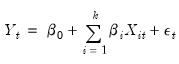 | (38.1) |
While this framework is typically sufficient for most applications, the requirement that coefficients be the same for all observations is quite restrictive and often violated in practice.
Alternatively, nonparametric modeling is agnostic as to the nature of the relationship between variables, assuming a general functional relationship between the dependent and explanatory variables:
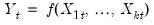 | (38.2) |
The flexibility of this specification comes at a cost as it can be difficult to interpret nonparametric estimates. For example, describing the marginal effects of a given variable upon

can be challenging.
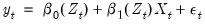
A flexible, middle ground between these two extremes is the functional coefficients model:
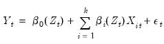 | (38.3) |
where the

are no longer simple coefficients, but are instead functions of the variable

. Here, the relationship is linear in variables, but non-linear in parameters. In contrast to the linear regression specification
Equation (38.1), the coefficients are no longer constant, but instead vary across observations. Non-linear phenomena are easily accommodated in this framework, coefficient relationships are dynamic, and interpretation of coefficient relationships is still intuitive.
Estimation of functional coefficient models is based on local polynomial regression, and incorporates two distinct techniques:
• Approximate the non-linear functions  using Taylor’s Theorem
 • Estimate local regressions where we penalize observations using a kernel function
The basic idea is that for each

of interest, we estimate a local regression with kernel weighted squared residuals. Then, estimating this regression for a set of

traces out the functional coefficients relationship.
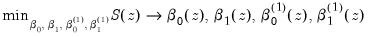
For example, suppose we have the single regressor functional coefficients model:
 | (38.4) |
We will approximate the coefficient functions

and

with a linear Taylor expansion at

. The resulting objective function is:
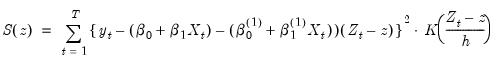 | (38.5) |
Minimizing this objective provides estimates of the coefficients at that point,
We may repeat this minimization for various

.
There are several points that we wish to emphasize:
• The functional coefficient estimate is a set of coefficients estimated at a corresponding set of points  .
. • The objective function depends on the kernel bandwidth 
.
• In this example, the objective contains twice as many coefficients as the base model to account for the presence of the first derivatives in the Taylor approximation. We are, however, typically interested only in  and
and  , and not in the corresponding
  and
and  .
. In this example, we employ a linear Taylor expansion, but EViews supports an arbitrary polynomial degree

in
Equation (38.5).
Bandwidth Selection
By far the most important step in estimating functional coefficient regressions is optimal selection of the bandwidth parameter

. At one extreme, when

, the functional coefficient estimator reduces to interpolating the data points in

(small bias, large variance). Alternatively, when

, the functional coefficient estimator reduces to the mean of

(large bias, small variance). Between these two extremes we may select a bandwidth that balances bias and variance.
Final Bandwidth
The bandwidth employed in
Equation (38.5) may be termed the estimation
final bandwidth. There are several popular methods used to select an optimal final bandwidth:
• : selects for the value which minimizes the integrated (or summed) mean squared error (IMSE) of the functional coefficient estimates, where the IMSE is defined as the average of the squared bias and variance contributions from each functional coefficient estimate at each function evaluation point

.
• : a leave-one-out variant of the IMSE bandwidth optimizer which minimizes the IMSE defined by averaging the squared bias and variance contributions from leave-one-out functional coefficients obtained at each observation evaluation point

.
• : computes the optimal bandwidth using a non-parametric AIC with non-parametric degrees of freedom. The idea stems from the Hastie and Tibshirani (1990) degrees of freedom smoothers literature, with the actual bandwidth methodology suggested in Cai, Fan and Yao (2000) and Cai (2003). Briefly, for each evaluation point

, and some bandwidth

, we estimate functional coefficients and use these to compute the standard error of the local polynomial regression residuals. The standard error and an estimated non-parametric degrees of freedom is then used to obtain a functional AIC value. The optimal bandwidth is obtained as the

which minimizes the AIC summed over the

.
In addition to these methods, you may employ any of the pilot methods described below which do not require preliminary functional coefficient estimates.
Pilot Bandwidth
It is important to note that the optimal estimation bandwidth estimators themselves require functional coefficient estimates to obtain standard errors, covariance matrix, and bias estimates. These preliminary estimates require their own
pilot bandwidth 
.
The pilot bandwidth is often determined using one of the following methods which do not depend on other bandwidths:
• : This method selects the pilot bandwidth using the asymptotic IMSE (AIMSE) Gaussian kernel as a reference. For a given bandwidth

, we compute the residual standard error of the functional coefficients regression obtained at each evaluation point

and sum these values. We search for the value of

which minimizes this sum, and use this value to obtain an optimal

value. For non-Gaussian kernels, the optimal bandwidth employs canonical kernel transformations as outlined in Marron and Nolan (1988), using the constants in Härdle,
et al.(1991, p. 76).
• A modified version of ROT which computes the objective by summing over the minimum of the residual standard error and

, where

is the inter-quartile range of the residuals.
• : A bandwidth estimator proposed by Fan and Gijbels (1995b). For each evaluation point

and bandwidth

, we compute a functional RSC value that depends on the residual variance, the polynomial degree of the functional coefficients estimation, and a number representing the effective number of local observations. The optional pilot bandwidth

is chosen to be the value that minimizes the sum of these values.
• The MMCV was proposed by Cai, Fan, and Yao (2000). The cross-validation procedure estimates, for each evaluation point

, a functional coefficient model using

different sub-series of lengths

and then computes the average mean square error (AMSE) from the

-step ahead forecast errors starting at observation

. The resulting

AMSE values are summed to form a functional objective value at

. The optimal pilot bandwidth

is the value that minimizes the sum of these functional objectives across the

.
Auxiliary Polynomial Degree
The estimation auxiliary regressions using pilot bandwidths also require the specification of a pilot polynomial degree. For reasons outlined in Fan and Gijbels (1995a) and Fan and Gijbels (1996), the pilot polynomial order

should exceed the estimation order

by an even integer,
.
Forecasting
Forecasting functional coefficient models, and in general, forecasting non-linear models, is considerably more difficult than forecasting linear models.
In particular, consider a series

is observed over the period

, and suppose a forecast is required for

for some integer

.
Point Forecasts
The optimal predictor is given by the familiar conditional expectation of the forecast value conditional on the observable information up to time

. We may evaluate this predictor in one of the following ways:
• : Following Fan and Yao (2003), a

-step ahead forecast can be obtained by substituting for the conditional expectation the corresponding fitted values
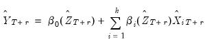 | (38.6) |
For static forecasting,  and
and  are set to the available actual values.
 For dynamic forecasting where the forecast sample evaluation points  or data
  , depend on the lagged endogenous variable, they may be set to the actual lagged endogenous
  or lagged forecast values
  as appropriate.
 • : For each forecast step

, the idea is to simulate a large number, say

of draws of

.
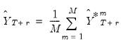
The  -step ahead forecast is obtained as the mean of the
  simulated series at that horizon of interest,
  | (38.7) |
where the simulated residual  is the
  -th draw (with replacement) from the within sample estimation residuals (Huang and Shen, 2004; Harvill and Ray, 2005).
 The  and
and  are functional coefficients estimates computed at the evaluation points
  using the original data
  .
. As with the Plug-in Method, the  and
and  are actual values, if available, for static forecasting. For dynamic forecasting,
  or
or  will be set to the actual lagged endogenous
  or lagged forecast values
  as appropriate.
 • : Similar to the approach, but with the simulated residual

drawn from a mean zero Gaussian distribution with standard deviation

obtained as the standard error of the estimation residuals.
• : In contrast to the Monte Carlo bootstrap methods which generate simulated values through the residual process, the full bootstrap forecast is the average of forecasts using bootstrap draws of the dependent variable.
As in the Monte Carlo - Bootstrap, for the  -th draw, we generate a bootstrap draw of the dependent variable
  for
for  using
using 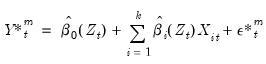 | (38.8) |
where the set of simulated residuals  , are a draw (with replacement) from the within sample estimation residuals.
 The  and
and  are functional coefficients estimates computed at the evaluation points
  using the original data
  .
. The data for the  -th simulation are then given by
  , where the
  and
and  are the original
  and
and  , or are lags of
  if the originals contain lags of
  .
. The corresponding  -step ahead individual forecast for the
  -th simulation is given by the fitted values:
 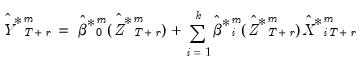 | (38.9) |
The  and
and  are functional coefficients estimated using the bootstrap simulation data
 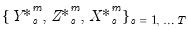 and evaluated at
  .
. Once again, in dynamic forecasting settings,  or
or  that depend on lagged endogenous variables will be set to actual values or lagged forecast values
  , as appropriate. For static forecasting,
  or
or  will be set to actuals.
 The forecast is obtained by averaging over the individual simulated forecasts:
 | (38.10) |
Note that the two bootstrap methods are not available in cases where the equation is specified using a dependent variable expression that is not normalizable.
Confidence Intervals
For forecasts that are obtained by Monte Carlo simulation methods, forecast confidence intervals may be obtained using the empirical distribution of the simulation results.
Monte Carlo forecast confidence intervals only consider residual uncertainty since resampling only involves a resampling from the residuals.
Confidence intervals for the full bootstrap are obtained by adapting the results in Davidson and Hinkley (1997) to functional coefficient models. Note that the full bootstrap introduces both coefficient and residual uncertainty into the calculation.