Technical Details
The optimization procedure uses a Newton (or quasi-Newton) based approach to optimization. In this approach, the first and second derivatives of the objective are used to form a local quadratic approximation to the objective function around the current value of the control parameters. The procedure then calculates the change in the control values that would maximize (or minimize) the objective if the objective function were to exactly follow the local approximation.
Mathematically, if the local approximation of the objective

around the control values

is:
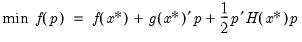 | (10.4) |
where

is the objective function,

is the gradient, and

is the Hessian, then the first-order conditions for a maximum give the following expression for the Newton step:
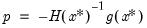 | (10.5) |
Note that this local approximation may become quite inaccurate as we move away from the current parameter values. At the full Newton step, the objective may improve by much less than the approximation suggests, or may even worsen. To deal with this possibility, the optimization procedure uses a trust region approach (More and Sorensen, 1983). In the trust region approach, the local quadratic approximation is only maximized within a limited neighborhood of the current control values, so that the change in control values at each step is not allowed to exceed a current maximum step size. We then evaluate the objective at the new proposed parameter values. If the local approximation appears to be accurate, the maximum allowed step size is increased. If the local approximation appears to be inaccurate, the maximum allowed step size is decreased. A step is only accepted when it results in a sufficiently large reduction in the objective relative to the reduction that was predicted by the local approximation.
Mathematically the constrained step can be written as:
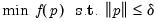 | (10.6) |
where

is the trust region maximum step size. In the case where the maximum step constraint is binding, typically the step has a solution
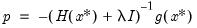 | (10.7) |
where

is chosen so that |

.
Note that the Newton approach will work best when the objective can be fitted reasonably well by a local quadratic approximation. This will not be the case if the function is discontinuous or has discontinuous first or second derivatives. In these cases, the procedure may be slow to find an optimum, and the final parameter values may end up adjacent to a discontinuity so that the results will need to be interpreted with caution.
Hessian Approximation
In the discussion above we assumed that the Hessian matrix of second derivatives of the objective with respect to the control parameters are readily available. In practice these derivatives will need to be approximated. The optimize procedure provides three different methods: numeric Hessian, Broyden-Fletcher-Goldfarb-Shanno (BFGS), outer-product of the gradients (OPG).
Numeric Hessian
The numeric Hessian approach approximates the Hessian using numeric derivatives. If analytic gradients are provided, the Hessian is based on taking numeric first derivatives of the analytic gradients. If analytic gradients are not provided, the Hessian is based on numeric second derivatives of the objective function.
You may specify the use of numeric Hessians by including the option “hess=numeric” option in the optimize command.
Note that calculating numeric second derivatives may require many evaluations of the objective function. In the case of numeric second derivatives, each Hessian approximation will require additional evaluations proportional to the square of the number of control parameters in the problem. For a large number of control parameters, this method may be quite slow.
Broyden-Fletcher-Goldfarb-Shanno (BFGS)
The Broyden-Fletcher-Goldfarb-Shanno (BFGS) method approximates the Hessian using an updating scheme where the previous iteration's approximation to the Hessian is adjusted after each step based on the observed change in the gradients.
The BFGS update makes as small a change as possible to the existing Hessian approximation so that it is compatible with the observed change in gradients, while ensuring that the approximation to the Hessian remains positive definite. (See Chapter 9 of Dennis and Schnabel (1983) for a detailed discussion.)
To specify the BFGS method, use the optimize command with the “hess=bfgs” option.
BFGS requires fewer objective function evaluations per step than computing a numeric Hessian, but may take more iterations to converge. Note that the BFGS approximation need not converge to the true Hessian at the optimized control parameter values, so it cannot be used for calculating the coefficient covariances in statistical problems. Note also that the iterations are started from a diagonal approximation to the Hessian.
Outer-product of Gradients (OPG)
For certain statistical problems, the Hessian can be approximated by a multiple of the sum of the outer products of the gradients (OPG) of individual contributions to the total objective with respect to the coefficients. In the case of least squares problems, this method is commonly referred to as the Gauss-Newton method. In maximum likelihood settings, this method is often referred to as the BHHH (Berndt, Hall, Hall, and Hausman, 1974) method.
In both settings, the approximations are based on the statistical idea that the expected value of the Hessian at the optimized parameter values is equal to a multiple of the expected value of the sum of the outer product of gradients and that the two will converge as the sample size becomes large. The asymptotic equivalence implies that these OPG approximations will be closer to the true Hessian when working with medium to large sample sizes and when coefficients are close to the true coefficient values.
You may select the OPG approximation using the “hess=opg” option.
Note that the OPG method may only be used when the objective is a set of least squares residuals (specified using the “ls” option) or a set of maximum likelihood contributions (specified using the “ml” option), since there is no reason to believe the approximation is valid for an arbitrary maximization or minimization objective.
OPG uses the same number of objective evaluations per step as BFGS, which is less than the number required for evaluating the numeric Hessian.
Step Method
Different step methods are supported by optimize, with each following a trust region approach, where the full Newton step is taken whenever the step is less than the current maximum step size, and a constrained step is taken when the full Newton step exceeds the current maximum step size. The methods differ in how the constrained step is taken. Note that in most cases, the choice of step method is less important than the selection of Hessian approximation.
Marquardt
The default Marquardt option closely follows the method outlined above where the constrained step is calculated by an iterative procedure that searches for a diagonal adjustment to the Hessian that makes the step size equal to the maximum allowed step size. The Marquardt step has the highest computational cost, although since for most statistical estimation most computation time is spent evaluating the objective rather than calculating an optimal step, this is unlikely to matter unless the number of controls is fairly large and the objective can be evaluated cheaply.
Dogleg
The dogleg method is a cheaper approximation to the trust region problem where the constrained step is calculated by combining a Newton step with a Cauchy step (a step in the direction of the scaled gradients that minimizes the local quadratic approximation to the objective). For both the Marquardt and dogleg steps, the direction of the step shifts away from the direction of the Newton step towards the direction of steepest descent as the trust region contracts, but the dogleg step uses a simple linear combination of the two steps to achieve this. When the dogleg step is used with a BFGS Hessian (the hess=bfgs option) approximation, the calculations required per iteration are proportional to the square rather than the cube of the number of parameters. This makes the dogleg step attractive if the number of control variables is very large and the objective can be evaluated cheaply.
Line-search
The line-search method is the simplest approach in which the constrained step is formed by proportionally scaling down the Newton step until it satisfies the maximum step size constraint. With this method, only the length of the step is changed as the trust region contracts, but not its direction. The line-search method is the cheapest method in terms of calculational cost but may be less robust, particularly when used with poor initial values.
Note that for both the dogleg and line-search algorithms, an adjustment will be made to the diagonal of the Hessian to ensure positive definiteness before calculating the Newton step. There is also special handling for non-positive definite matrices in the Marquardt step following the method outlined in More and Sorensen (1983).
Scaling
The Newton step is theoretically invariant to both the scale of the objective and the scale of the control variables since any changes to the gradients and the Hessian cancel each other out in the expression for the Newton step. In practice, numerical issues may cause the equivalence to be inexact. Additionally, the constrained trust region steps do not have the invariance property unless scaling is applied to the control variables when calculating a constrained step.
By default, the optimization procedure scales automatically using the square root of the maximum observed value of the second derivative (curvature) of each control parameter. This makes the procedure theoretically invariant to the scaling of the variables.
In most cases you should leave the default scaling turned on, but in cases where the Hessian approximation may be unreliable, scaling may be switched off using the “scale=none” option. When scaling is switched off, you may wish to define your objective so that equal size changes to each control variable will have a similar order of magnitude of impact on the objective.
Optimization Termination
The optimization process will terminate immediately if the initial control parameters contain missing values, the objective function, or if provided, the analytical gradients cannot be evaluated at the starting parameter values.
Once the optimization procedure begins, it will proceed even if numerical errors (such as taking the log of a negative number) prevent the objective function from being evaluated at a trial step. An objective with missing values will be taken as indicating that the control values are invalid, and the optimization will step back from the problematic values.
Note that you should always define the objective to return NA values for bad control values since returning an arbitrary value may make numeric derivatives unreliable at points close to the invalid region.
The optimization procedure will terminate when:
• An unconstrained Newton step improved the objective and the length of the step was less than the specified convergence tolerance.
• A constrained step failed to improve the objective and the maximum allowed step size for the next iteration was decreased to become less than the specified convergence tolerance.
• The maximum number of iterations (successful steps) was reached without one of the above criteria being met.
When the procedure terminates for a condition other than the maximum iterations being reached, the procedure checks the gradients and curvature of the objective to see whether the first and second order conditions for an optimum appear to be satisfied. If the conditions are not met, the optimization will be considered to have failed. There are a variety of reasons that failure may occur:
• The objective may have no optimum value, but just gradually flatten out as a control variable becomes very large or small.
• The objective may not be defined for some values of the control parameters but may improve as we approach these values. This will cause the optimization to stall with control variables very close to the invalid region, but with non-zero gradients at the final control values.
• There may be values for some controls which make other controls included in the optimization have little or no impact on the objective, so that both the gradients and the elements of the Hessian corresponding to the variables gradually become zero as the optimization progresses.
• The control variables may 'collapse' so that two or more controls are serving the same role in the objective and their individual effect cannot be separated. This will result in a Hessian that is numerically singular since changes in one control can be exactly offset by changes in one or more of the other controls without changing the objective. (For statistical problems, this implies that the coefficients are unidentified).
In all these cases, a useful approach is to carefully consider starting values so that the initial values for the controls are as close as possible to what you believe the optimum values might be. You should also avoid starting values that are close to any regions in which the objective function cannot be evaluated. If the optimization continues to report problems from a wide range of starting values, this may indicate that your optimization problem is not well defined.
Successful convergence does not guarantee that the optimization procedure has found the global optimum of the function. The optimization procedure only tests whether the final point appears to satisfy the conditions necessary for a local optimum. In cases where more than one local optimum may exist, the optimization procedure may converge to different final values depending on what starting values are used.
Note that when the optimization completes successfully (no error is reported) the last call to the subroutine that calculates the objective will always be with the control parameters set to the optimized values. (An additional final call to the subroutine will be made in situations where this is not already the case). This guarantees that any intermediate results saved inside the subroutine will also be left at their optimized results after the optimization is complete.