(36.1)
| (36.1) |
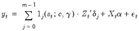
 is a (0, 1) indicator for regime that depends on the observed variable
  , where
  represents one or more thresholds and
  is a threshold slope parameter. Note that we have divided the regressors into two groups—
  variables whose coefficients vary across the
  regimes, and
  variables with coefficients that are regime invariant.
 , as using the fact that
  for exactly one
  , we may rewrite the discrete TR equation as:
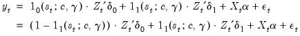 | (36.2) |
 that returns values between 0 to 1. Then we have
 | (36.3) |
 has different properties as
  ,
,  , and
, and  , depending on the specific functional form.
  and the selection of a transition function
  . For a given
  and
and  , we may estimate the regression parameters
  and the threshold values and slope
  via nonlinear least squares. Additionally, given a list of candidate variables for
  , we can select a threshold variable using model selection techniques.
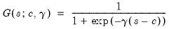 | (36.4) |
 | (36.5) |
 | (36.6) |
 | (36.7) |
 in all cases.
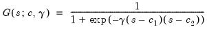
 so that the two regimes correspond to high and low values of the threshold variable. The threshold value
  determines the point at which the regimes are equally weighted, while
  controls the speed and smoothness of the transition. As
  , the transition function approaches the indicator function and the model approaches the discrete threshold model.
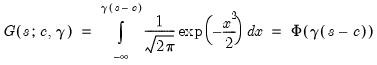
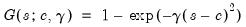
 from the threshold
  . Furthermore,
  when
when  , and
, and  approaches 1 as
  and
and  . The ESTR model does not nest the discrete TR model since, as
  or
or  , the specification becomes linear since
  approaches a constant function returning 0 or 1.
 with distinct
  ,
,  approaches 1 for
  and
and  , and
, and  approaches 0 for
  in-between. Thus, the L2STR model nests a three-regime discrete TR model where the outer regimes have a common linear specification.
 ,
,  attains its minimum value at
  with a non-zero value.
 , see van Dijk, Teräsvirta, and Franses (2002) who offer extensive commentary on the properties of these transition functions and provide concrete examples of their use in empirical settings.
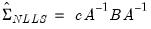 | (36.8) |
 is an estimate of the information,
  is the variance of the residual weighted gradients, and
  is a scale parameter.
 . Then we have
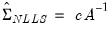 | (36.9) |
 is an estimator of the residual variance (with or without degree-of-freedom correction).
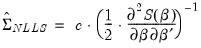
  using the outer-product of the gradients (OPG) of the error function or the one-half of the Hessian matrix of second derivatives of the sum-of-squares function:
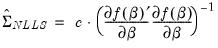 | (36.10) |
 | (36.11) |
 and
and  , and employ a White or HAC sandwich estimator for the coefficient covariance as in
“Robust Standard Errors”.
, and employ a White or HAC sandwich estimator for the coefficient covariance as in
“Robust Standard Errors”.