Static graphs display data for a fixed range of observations. That range may consist of a single observation or multiple observations, but it does not change. With animated graphs, you can dynamically adjust the range of data and display how the data change over a given interval. Animated graphs allow viewers to see how data transition from one period to another or how it compares between periods.

An animated graph is nothing more than multiple static graphs displayed one after another. This gives the impression of motion. To animate a graph, either the axis range, data range, or both must change. When changing the axis or data range, you must adjust one or more of the following: axis min/max and data min/max values. Additionally, you must determine by how much to adjust those value. Depending on the increments used, graphs can appear to move, grow, or both. Note that frozen graphs or graphs that do not update cannot be animated.

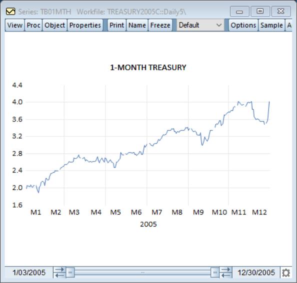
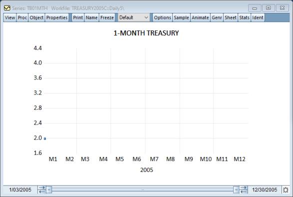
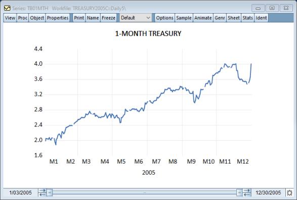
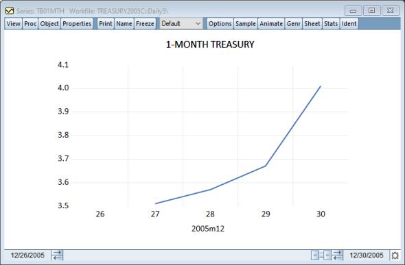
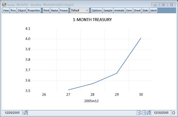
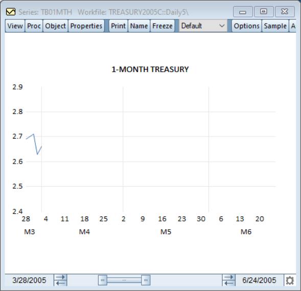
From the Treasurey2005c.wf1 workfile located in Graphing Data Example Files directory we display a line graph of the 1-Month Treasury bond rate (tb01mth):

With animated graphs you can view how the bond rate changes as a function of time. Press the Animate button in the toolbar and the animation dialog will appear. Next, press the Show Details button.

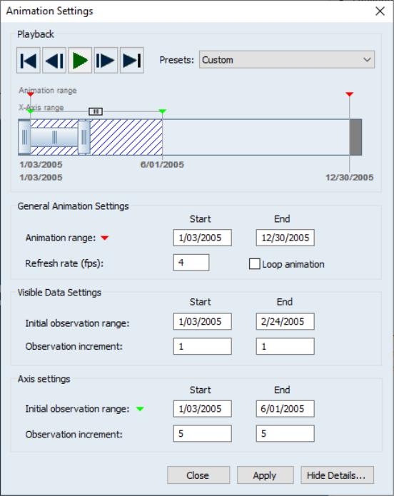
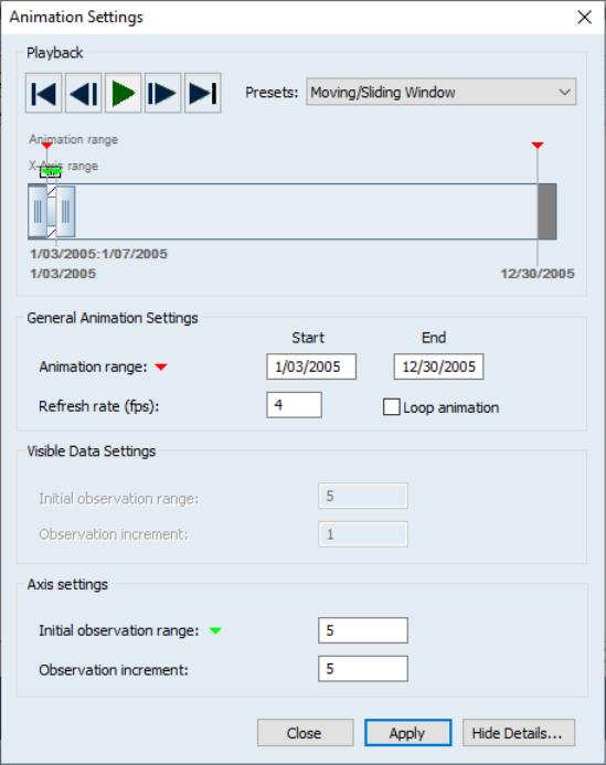
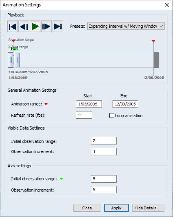
The animation dialog is split into four sections. Each section controls a different aspect of the animation. These are Playback, General Animation Settings, Visible Data Settings, and Axis Settings. The playback settings allow you to start and stop the animation, choose one of the predefined animation types, and give a visible representation of how the graph will be animated.

The first area is the control area with five buttons: jump to animation start (first frame), move to previous frame, play/pause animation, move to next frame, jump to animation end (last frame). To the right of the control buttons is the Presets: combo box. Here is where you can choose from a list of predefined animation types. Details on these types will be discussed later.

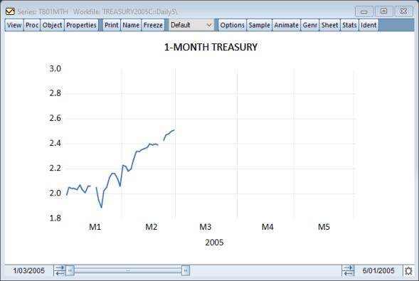
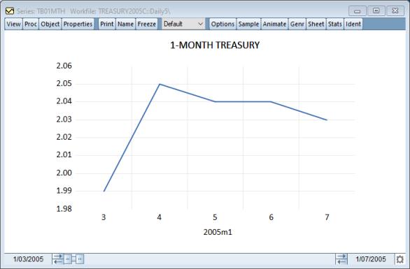
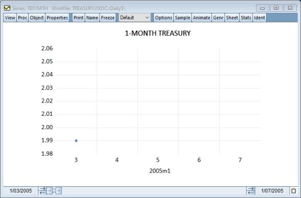
At the bottom of the Playback section is the animation viewer. The viewer shows the relationship between an individual frame and the entire animation sequence. In it you can identify observations where the animation should start and end. This is called the animation range and is denoted by red arrows at the top of the preview. The text representation of the animation range can be found at the bottom of the viewer and beneath the corresponding red arrow. Just below the animation range arrows are the green X-Axis range arrows. These denote the current x-axis range of the graph for the current frame. The text representation of the axis range can be found above the animation range text and below the corresponding axis arrow. In the center of the viewer there are two rectangular boxes. These boxes represent the data that is being viewed within the axis range. Using the figure above, the animation will start on January 3, 2005 and stop at December 31, 2005. The initial graph axis spans January 3, 2005 to June 1, 2005, and the viewable data spans January 1, 2005 to February 24, 2005. The result of these settings can be seen in the figure below.

The second section of the dialog contains the animation settings that are independent of the type. These include the animation range, refresh rate (how many frames are shown per second) and whether the animation should reset when the end is reached.

The third section contains the Visible Data Settings. The first set of edit controls here determines the viewable data range for the first frame of the animation. The second line of controls dictate how the data range will change on subsequent animation frames. In our example, the observation increment for both the start and end is 1. Since our initial data range is January 3, 2005 to February 24, 2005, the data range of the next frame will be January 4, 2004 to February 25, 2005. The range for the third frame will be January 5, 2004 to February 26, 2005. This continues for subsequent frames.

The fourth section of the dialog contains the graph Axis Settings. Here is where you will set the axis range for the first frame of the animation. Just below that are the start and end axis increment values that control how the axis will change during the animation. Depending on the presets selected, the third (data) section or fourth (axis) section may be greyed out.

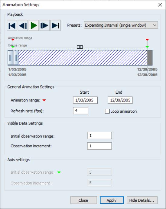
There are four selections in the Presets: combo box: Expanding Interval (single window), Moving/Sliding Window, Expanding Interval with Moving Window, and Custom. Expanding Interval has a fixed axis range and variable data range. In the first frame of the animation, the data range may start and end with the first observation (this is adjustable). By the end of the animation, the data range will match the axis range. Using this mode, you can see how the bond rate changes as time progresses. By default, if we choose the Expanding Interval (single window) type, the dialog and graph will appear as:

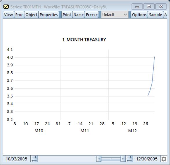
The x-axis for this graph is the full workfile range, January 1 to December 31, 2005. During the animation, one observation will be added to the end of the data range for each frame. The number of observations added can be changed by editing the Observation Increment edit box. Next, if we press the play button in the dialog the graph will expand the data range until it matches the axis range, yielding the figure below:

Unlike the Expanding Intervals where the data grows, Moving/Sliding Window graphs slices of time. In this case, the data range always matches the axis range and the ranges are of fixed observation width. Also, unlike Expanding Intervals the axis range changes from frame to frame. Switching the Preset to Moving/Sliding Window, the dialog appears as:

And the graph will by produce:

In this example, we can see a week's worth of data. For each subsequent frame, the axis will advance by five observations as specified in the Observation Increment edit box. This is equivalent to a week in our 5-day weekly workfile. Subsequently we will continue to only see a week's worth of data, moving through each week over time. Notice the axis is moving and changing in every frame, while for Expanding Intervals the axis was fixed and the data were growing. At the end of a Moving/Sliding Window animation, the last frame will contain the last week of data from the workfile.

The third preset is the Expanding Interval with Moving Window. An Expanding Interval with Moving Window graph is a combination of the two previous animation types. The data range will initially match the first axis range observation and expands during the animation. The axis range is of fixed size but once the data range matches the axis range, the axis range will advance.

As time progresses, the data range will expand by one, as specified in the Visible Data Range - Observation increment, until it matches the axis range.

Once the ranges match, the axis range will advance by the value specified in the Axis Settings - Observation increment edit box. At this time, the data range will also reset to the beginning of the new axis range.

This process will continue until the axis range reaches the end of the animation and the data range matches the final axis range.

Lastly, if the predefined types do not suit your needs, we have also provided the Custom graph animation type. The custom type offers a lot more customization that isn't available in the previously mentioned preset types. For example, in the previous preset types the data range starts always match the axis range starts and the data range ends will either match the axis starts or the axis ends. Additionally, the data range starts are fixed and never change. The axis start and end increments are also equal. However, when using the Custom type, you may remove these restrictions. The data range does not need to start at the same observation as the axis start and the increments for the starts do not need to match the ends or be zero.

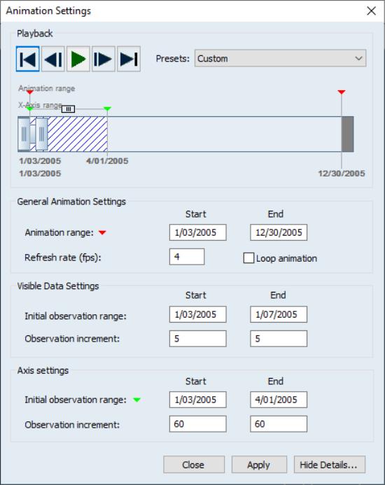
We will next describe an example to demonstrate what can be achieved using the Custom type. The example is similar to the Expanding Interval with Moving Window type. We are going to create an animation where the axis will span three months (one quarter), and only one week of data, from Monday to Friday, will be visible.

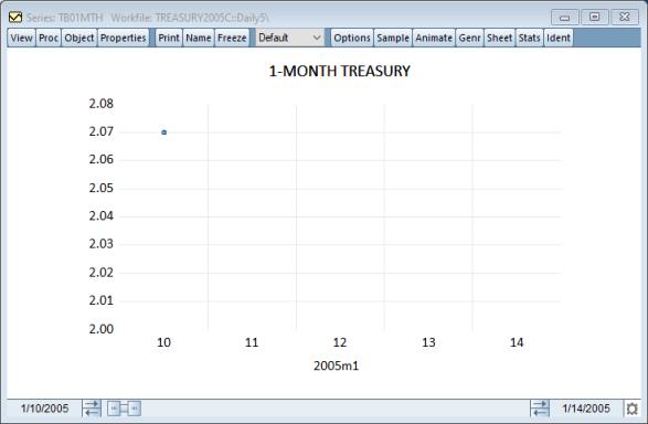
In the Visible Data Settings, we set the start to Monday January 3rd and the end to Friday January 7th. For the Observation increment: we set both the start and end to five. This will advance the start to the next Monday and the end to the next Friday, since this is a 5-day weekly workfile. We also set the axis range from January 3rd to April 1st, or one quarter. Once the data end reaches the axis end, the axis range will then advance sixty observations (one quarter). The initial graph will look like this:

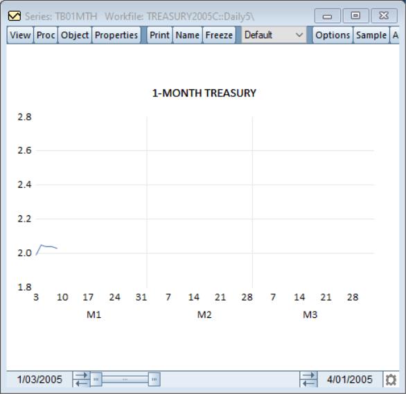
Eventually the graph will look like this:

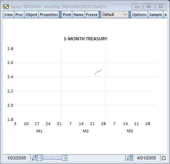
And then this:

And finally this: