Opens a program file, or text (ASCII) file.
This command should be used to open program files or text (ASCII) files for editing.
You may also use the command to open workfiles or databases. This use of the
open command for this purposes is provided for backward compatibility. We recommend instead that you use the new commands
wfopen and
pageload to open a workfile, and
dbopen to open databases.
Syntax
open(options) [path\]file_name
You should provide the name of the file to be opened including the extension (and optionally a path), or the file name without an extension but with an option identifying its type. Specified types always take precedence over automatic type identification. If a path is not provided, EViews will look for the file in the default directory.
Files with the “.PRG” extension will be opened as program files, unless otherwise specified. Files with the “.TXT” extension will be opened as text files, unless otherwise specified.
For backward compatibility, files with extensions that are recognized as database files are opened as EViews databases, unless an explicit type is specified. Similarly, files with the extensions “.WF” and “.WF1”, and foreign files with recognized extensions will be opened as workfiles, unless otherwise specified.
All other files will be read as text files.
Options
p | Open file as program file. |
t | Open file as text file. |
type=arg (“prg” or “txt”) | Specify text or program file type using keywords. |
Examples
open finfile.txt
opens a text file named “Finfile.TXT” in the default directory.
open "c:\program files\my files\test1.prg"
opens a program file named “Test1.PRG” from the specified directory.
open a:\mymemo.tex
opens a text file named “Mymemo.TEX” from the A: drive.
Cross-references
See
wfopen and
pageload for commands to open files as workfiles or workfile pages, and
dbopen for opening database files.
Find the solution to a user-defined optimization problem.
The optimize command calls the EViews optimizer to find the optimal control values for a subroutine defined elsewhere in the program file or files.
Syntax
optimize(options) subroutine_name(arguments)
You should follow the optimize command keyword with options and subroutine_name, the name of a defined subroutine in your program (or included programs).
The subroutine must contain at least two arguments.
By default EViews will interpret the first argument as the output of the subroutine and will use it as the value to optimize. If the objective contains more than one value, as in a series or vector, EViews will optimize the sum of the values. The second argument is, by default, used to define the control parameters for which EViews will find the optimal values.
Since the objective and controls are defined by a standard EViews subroutine, the arguments of the subroutine may correspond to numbers, strings, and various EViews objects such as series, vectors, scalars.
Options
Optimization Objective and Controls
The default optimization objective is to maximize the first argument of the subroutine. You may use the following optimization options to change the optimization objective and to specify the coefficients (control parameters):
max [=integer] | Maximize the subroutine objective or sum of the values of the subroutine objective (default). By default the first argument of the subroutine is used as the maximization objective. You may change the objective to another argument by specifying an integer argument location. |
min [=integer] | Minimize the subroutine objective or sum of the values of the subroutine objective. By default the first argument of the subroutine is used as the minimization objective. You may change the objective to another argument by specifying an integer argument location. |
ls [=integer] | Perform least squares minimization of the sum of squared values of the subroutine objective. (The objective argument cannot be a scalar value when using this option.) By default the first argument of the subroutine is used as the minimization objective. You can change the objective to another argument by specifying an integer argument location. |
ml [=integer] | Perform maximum likelihood estimation of the sum of the values of the subroutine objective. (The objective argument cannot be a scalar value when using this option.) By default the first argument of the subroutine is used as the maximization objective. You can change the objective to another argument by specifying an integer argument location. Note that the “ml” option specifies the same optimization as when using the “max” option, but permits a different set of Hessian matrix choices. |
coef=integer (default = 2) | Specify the argument number of the function that contains the coefficient controls for the optimization. If the argument is a vector or matrix, each element of the vector or matrix will be treated as a coefficient. If the argument is a series, each element of the series within the current workfile sample will be treated as a coefficient. The default value is 2 so that the second argument is assumed to contain the coefficient controls. |
Optimization Options
grads=integer | Specifies an argument number corresponding to analytic gradients for each of the coefficients. If this option is not specified, gradients are evaluated numerically. Available for “ls” and “ml” estimation. • If the objective argument is a scalar, the gradient argument should be a vector of length equal to the number of elements in the coefficient argument. • If the objective argument is a series, the gradient argument should be a group object containing one series per element of the coefficient argument. The series observations should contain the corresponding derivatives for each observation in the current workfile sample. • For a vector objective, the gradient argument should be a matrix with number of rows equal to the length of the objective vector, and columns equal to the number of elements in the coefficient argument. • “grad=” may not be specified if the objective is a matrix. |
hess=arg | Specify the type of Hessian approximation: “numeric” (numerical approximation), “bfgs” (Broyden–Fletcher–Goldfarb–Shanno), or “opg” (outer product of gradients, or BHHH). “opg” is only available when using “ls” or “ml” optimization. The default value is “bfgs” unless using “ls” optimization, which defaults to “opg”. |
step=arg (default_= “marquardt”) | Set the step method: “marquardt”, “dogleg” or “linesearch”. |
scale=arg | Set the scaling method: “maxcurve” (default), or “none”. |
m=int | Set the maximum number of iterations |
c=number | Set the convergence criteria. |
trust=number (default=0.25) | Sets the initial trust region size as a proportion of the initial control values. Smaller values of this parameter may be used to provide a more cautious start to the optimization in cases where larger steps immediately lead into an undesirable region of the objective. Larger values may be used to reduce the iteration count in cases where the objective is well behaved but the initial values may be far from the optimum values. |
deriv=high | Always use high precision numerical derivatives. Without this option, EViews will start by using lower precision derivatives, and switch to higher precision as the optimization progresses. |
feps=number (default=2.2e-16) | Set the expected relative accuracy of the objective function. The value indicates what fraction of the observed objective value should be considered to be random noise. |
noerr | Turn off error reporting. |
finalh=name | Save the final Hessian matrix into the workfile with name name. For “hess=bfgs”, the final Hessian will be based on numeric derivatives rather than the BFGS approximation used during the optimization since the BFGS approximation need not converge to the true Hessian. |
Examples
The first example estimates a regression model using maximum likelihood. The subroutine LOGLIKE first computes the regression residuals using the coefficients in the vector BETA along with the dependent variable series given by DEP and the regressors in the group REGS.
subroutine loglike(series logl, vector beta, series dep, group regs)
series r = dep - beta(1) - beta(2)*regs(1) - beta(3)*regs(2) - beta(4)*regs(3)
logl = @log((1/beta(5))*@dnorm(r/beta(5)))
endsub
series LL
vector(5) MLCoefs
MLCoefs = 1
MLCoefs(5) = 100
optimize(ml=1, finalh=mlhess, hess=numeric) loglike(LL, MLCoefs, y, xs)
The optimize command instructs EViews to use the LOGLIKE subroutine for purposes of maximization, and to use maximum likelihood to maximize the sum (over the workfile sample) of the LL series with respect to the five elements of the vector MLCOEFS. EViews employs a numeric approximation to the Hessian in optimization, and saves the final estimate in the workfile in the sym object MLHESS.
Notice that we specify initial values for the MLCOEFS coefficients prior to calling the optimization routine.
Our second example recasts the estimation above as a least squares optimization problem, and illustrates the use of the “grads=” option to employ analytically computed gradients defined in the subroutine.
subroutine leastsquareswithgrads(series r, vector beta, group grads, series dep, group regs)
r = dep - beta(1) - beta(2)*regs(1) - beta(3)*regs(2) - beta(4)*regs(3)
grads(1) = 1
grads(2) = regs(1)
grads(3) = regs(2)
grads(4) = regs(3)
endsub
series LSresid
vector(4) LSCoefs
lscoefs = 1
series grads1
series grads2
series grads3
series grads4
group grads grads1 grads2 grads3 grads4
optimize(ls=1, grads=3) leastsquareswithgrads(LSresid, lscoefs, grads, y, xs)
Note that for a linear least squares problem, the derivatives of the coefficients are trivial - the regressors themselves (and a series of ones for the constant).
The next example uses matrix computation to obtain an optimizer objective that finds the solution to the same least squares problem. While the optimizer is not a solver, we can trick it into solving that equation by creating a vector of residuals equal to
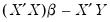
, and asking the optimizer to find the values of

that minimize the square of those residuals:
subroutine local matrixsolve(vector rvec, vector beta, series dep, group regs)
stom(regs, xmat)
xmat = @hcat(@ones(100), xmat)
stom(dep, yvec)
rvec = @transpose(xmat)*xmat*beta - @transpose(xmat)*yvec
rvec = @epow(rvec,2)
endsub
vector(4) MSCoefs
MSCoefs = 1
vector(4) rvec
optimize(min=1) matrixsolve(rvec, mscoefs, y, xs)
The first few lines of the subroutine convert the input dependent variable series and regressor group into matrices. Note that the regressor group does not contain a constant term upon input, so we append a column of ones to the regression matrix XMAT, using the @hcat command.
Lastly, we define a subroutine containing the quadratic form, and use the optimize command to find the value that minimizes the function:
subroutine f(scalar !y, scalar !x)
!y = 5*!x^2 - 3*!x - 2
endsub
scalar in = 0
scalar out = 0
optimize(min) f(out, in)
The subroutine F calculates the simple quadratic formula:
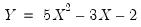 | (17.1) |
which attains a minimum of -2.45 at an IN value of 0.3.
Cross-references