Special Equation Expressions
EViews provides you with special expressions that may be used to specify and estimate equations with PDLs, dummy variables, or ARMA errors. We consider here terms for incorporating PDLs and dummy variables into your equation, and defer the discussion of ARMA estimation to
“Time Series Regression”.
Polynomial Distributed Lags (PDLs)
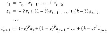
A distributed lag is a relation of the type:
 | (21.1) |
The coefficients

describe the lag in the effect of

on

. In many cases, the coefficients can be estimated directly using this specification. In other cases, the high collinearity of current and lagged values of

will defeat direct estimation.
You can reduce the number of parameters to be estimated by using polynomial distributed lags (PDLs) to impose a smoothness condition on the lag coefficients. Smoothness is expressed as requiring that the coefficients lie on a polynomial of relatively low degree. A polynomial distributed lag model with order

restricts the

coefficients to lie on a

-th order polynomial of the form,
 | (21.2) |
for
, where

is a pre-specified constant given by:
 | (21.3) |
The PDL is sometimes referred to as an Almon lag. The constant

is included only to avoid numerical problems that can arise from collinearity and does not affect the estimates of

.
This specification allows you to estimate a model with

lags of

using only

parameters (if you choose

, EViews will return a “Near Singular Matrix” error).
If you specify a PDL, EViews substitutes
Equation (21.2) into
(21.1), yielding,
 | (21.4) |
where:
 | (21.5) |
Once we estimate

from
Equation (21.4), we can recover the parameters of interest

, and their standard errors using the relationship described in
Equation (21.2). This procedure is straightforward since

is a linear transformation of

.
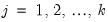
The specification of a polynomial distributed lag has three elements: the length of the lag

, the degree of the polynomial (the highest power in the polynomial)

, and the constraints that you want to apply. A near end constraint restricts the one-period lead effect of

on

to be zero:
 | (21.6) |
A far end constraint restricts the effect of

on

to die off beyond the number of specified lags:
 | (21.7) |
If you restrict either the near or far end of the lag, the number of

parameters estimated is reduced by one to account for the restriction; if you restrict both the near and far end of the lag, the number of

parameters is reduced by two.
By default, EViews does not impose constraints.
How to Estimate Models Containing PDLs
You specify a polynomial distributed lag by the pdl term, with the following information in parentheses, each separated by a comma in this order:
• The name of the series.
• The lag length (the number of lagged values of the series to be included).
• The degree of the polynomial.
• A numerical code to constrain the lag polynomial (optional):
1 | constrain the near end of the lag to zero. |
2 | constrain the far end. |
3 | constrain both ends. |
You may omit the constraint code if you do not want to constrain the lag polynomial. Any number of pdl terms may be included in an equation. Each one tells EViews to fit distributed lag coefficients to the series and to constrain the coefficients to lie on a polynomial.
For example, the commands:
ls sales c pdl(orders,8,3)
fits SALES to a constant, and a distributed lag of current and eight lags of ORDERS, where the lag coefficients of ORDERS lie on a third degree polynomial with no endpoint constraints. Similarly:
ls div c pdl(rev,12,4,2)
fits DIV to a distributed lag of current and 12 lags of REV, where the coefficients of REV lie on a 4th degree polynomial with a constraint at the far end.
The pdl specification may also be used in two-stage least squares. If the series in the pdl is exogenous, you should include the PDL of the series in the instruments as well. For this purpose, you may specify pdl(*) as an instrument; all pdl variables will be used as instruments. For example, if you specify the TSLS equation as,
sales c inc pdl(orders(-1),12,4)
with instruments:
fed fed(-1) pdl(*)
the distributed lag of ORDERS will be used as instruments together with FED and FED(–1).
Polynomial distributed lags cannot be used in nonlinear specifications.
Example
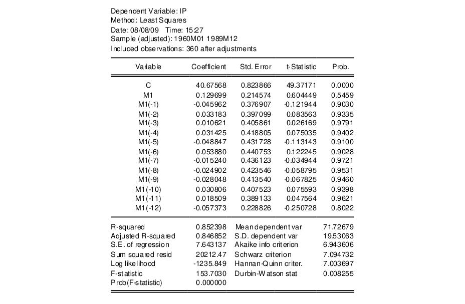
We may estimate a distributed lag model of industrial production (IP) on money (M1) in the workfile “Basics.WF1” by entering the command:
ls ip c m1(0 to -12)
which yields the following results:
Taken individually, none of the coefficients on lagged M1 are statistically different from zero. Yet the regression as a whole has a reasonable

with a very significant
F-statistic (though with a very low Durbin-Watson statistic). This is a typical symptom of high collinearity among the regressors and suggests fitting a polynomial distributed lag model.
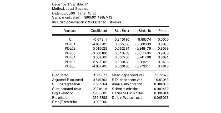
To estimate a fifth-degree polynomial distributed lag model with no constraints, set the sample using the command,
smpl 1959m01 1989m12
then estimate the equation specification:
ip c pdl(m1,12,5)
by entering the expression in the dialog and estimating using .
The following result is reported at the top of the equation window:
This portion of the view reports the estimated coefficients

of the polynomial in
Equation (21.2). The terms PDL01, PDL02, PDL03, …, correspond to

in
Equation (21.4).
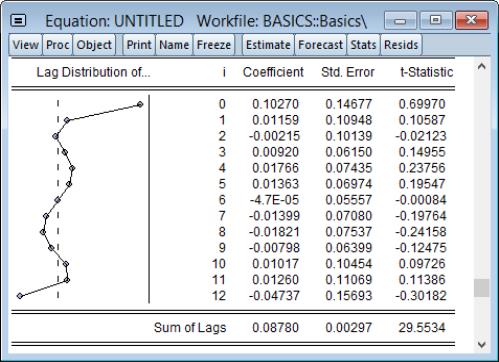
The implied coefficients of interest

in equation (1) are reported at the bottom of the table, together with a plot of the estimated polynomial:
The reported at the bottom of the table is the sum of the estimated coefficients on the distributed lag and has the interpretation of the long run effect of M1 on IP, assuming stationarity.
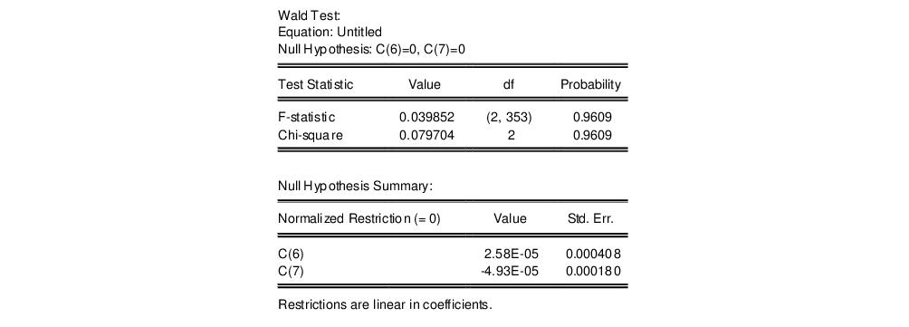
Note that selecting for an equation estimated with PDL terms tests the restrictions on

, not on

. In this example, the coefficients on the fourth- (PDL05) and fifth-order (PDL06) terms are individually insignificant and very close to zero. To test the joint significance of these two terms, click and enter:
c(6)=0, c(7)=0
in the Wald Test dialog box (see
“Wald Test (Coefficient Restrictions)” for an extensive discussion of Wald tests in EViews). EViews displays the result of the joint test:
There is no evidence to reject the null hypothesis, suggesting that you could have fit a lower order polynomial to your lag structure.
Automatic Categorical Dummy Variables
EViews equation specifications support expressions of the form:
@expand(ser1[, ser2, ser3, ...][, drop_spec])
When used in an equation specification, @expand creates a set of dummy variables that span the unique integer or string values of the input series.
For example consider the following two variables:
• SEX is a numeric series which takes the values 1 and 0.
• REGION is an alpha series which takes the values “North”, “South”, “East”, and “West”.
The equation list specification
income age @expand(sex)
is used to regress INCOME on the regressor AGE, and two dummy variables, one for “SEX=0” and one for “SEX=1”.
Similarly, the @expand statement in the equation list specification,
income @expand(sex, region) age
creates 8 dummy variables corresponding to:
sex=0, region="North"
sex=0, region="South"
sex=0, region="East"
sex=0, region="West"
sex=1, region="North"
sex=1, region="South"
sex=1, region="East"
sex=1, region="West"
Note that our two example equation specifications did not include an intercept. This is because the default @expand statements created a full set of dummy variables that would preclude including an intercept.
You may wish to drop one or more of the dummy variables. @expand takes several options for dropping variables.
The option @dropfirst specifies that the first category should be dropped so that:
@expand(sex, region, @dropfirst)
no dummy is created for “SEX=0, REGION="North"”.
Similarly, @droplast specifies that the last category should be dropped. In:
@expand(sex, region, @droplast)
no dummy is created for “SEX=1, REGION="WEST"”.
You may specify the dummy variables to be dropped, explicitly, using the syntax @drop(val1[, val2, val3,...]), where each argument specified corresponds to a successive category in @expand. For example, in the expression:
@expand(sex, region, @drop(0,"West"), @drop(1,"North"))
no dummy is created for “SEX=0, REGION="West"” and “SEX=1, REGION="North"”.
When you specify drops by explicit value you may use the wild card “*” to indicate all values of a corresponding category. For example:
@expand(sex, region, @drop(1,*))
specifies that dummy variables for all values of REGION where “SEX=1” should be dropped.
We caution you to take some care in using @expand since it is very easy to generate excessively large numbers of regressors.
@expand may also be used as part of a general mathematical expression, for example, in interactions with another variable as in:
2*@expand(x)
log(x+y)*@expand(z)
a*@expand(x)/b
Also useful is the ability to renormalize the dummies
@expand(x)-.5
Somewhat less useful (at least its uses may not be obvious) but supported are cases like:
log(x+y*@expand(z))
(@expand(x)-@expand(y))
As with all expressions included on an estimation or group creation command line, they should be enclosed in parentheses if they contain spaces. Thus, the following expressions are valid,
a*expand(x)
(a * @expand(x))
while this last expression is not,
a * @expand(x)
Example
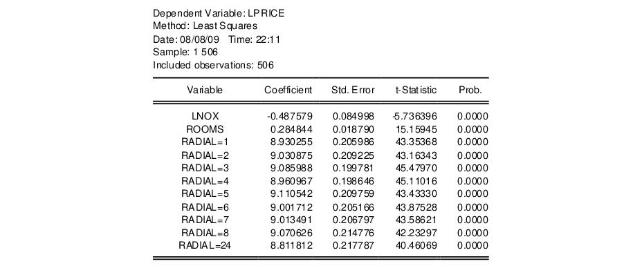
Following Wooldridge (2000, Example 3.9, p. 106), we regress the log median housing price, LPRICE, on a constant, the log of the amount of pollution (LNOX), and the average number of houses in the community, ROOMS, using data from Harrison and Rubinfeld (1978). The data are available in the workfile “Hprice2.WF1”.
We expand the example to include a dummy variable for each value of the series RADIAL, representing an index for community access to highways. We use @expand to create the dummy variables of interest, with a list specification of:
lprice lnox rooms @expand(radial)
We deliberately omit the constant term C since the @expand creates a full set of dummy variables. The top portion of the results is depicted below:
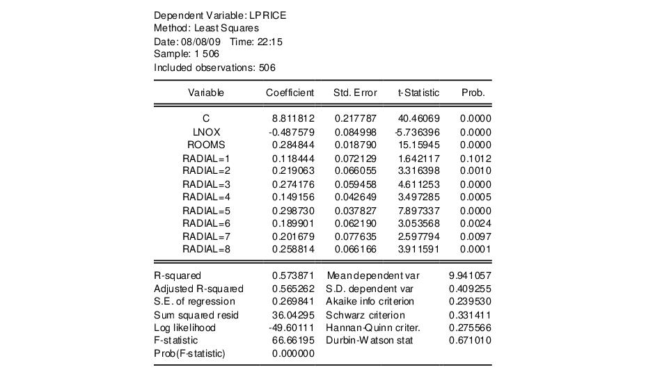
Note that EViews has automatically created dummy variable expressions for each distinct value in RADIAL. If we wish to renormalize our dummy variables with respect to a different omitted category, we may include the C in the regression list, and explicitly exclude a value. For example, to exclude the category RADIAL=24, we use the list:
lprice c lnox rooms @expand(radial, @drop(24))
Estimation of this specification yields: