Structural (Identified) VARs
A structural VAR (SVAR) uses additional identifying restrictions and estimation of structural matrices to transform VAR errors into uncorrelated structural shocks. Obtaining structural shocks is central to a wide range of VAR analysis, including impulse response, forecast variance decomposition, historical decomposition, and other forms of causal analysis. See, for example, Amisano and Giannini (1997), Martin, Hurn and Harris (2013).
We begin with the SVAR specification
 | (44.30) |
where

, all of the

, and

are the structural coefficients, and the

are the orthonormal unobserved structural innovations with
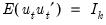
.
It is easy to see the relationship between the SVAR specification and the corresponding reduced-form VAR. Assuming that

is invertible, we have:
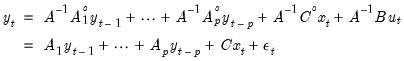 | (44.31) |
so the reduced-form lag matrices

and

, and the reduced form error structure is given by
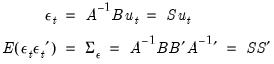 | (44.32) |
where

.
SVAR estimation uses estimates

obtained from the reduced form VAR, the short-run covariance relationships and any restrictions in
Equation (44.32), and long-run restrictions on the accumulated impulse responses (as described below), to identify and estimate the model. The challenge in SVAR estimation is that there are only

moments in

and more than

elements in

and

, or in

so that those matrices are not identified unless additional restrictions are provided.
SVAR Restrictions
Prior knowledge and theory will often suggest restrictions on structural matrices, allowing you to identify and estimate the parameters of the SVAR. EViews allows you to specify restrictions in different ways, with support for restrictions using two different short-run representations, and restrictions on the long-run impulse-responses.
Our discussion of SVAR restrictions and estimation is necessarily brief. We encourage those interested in greater detail to consult Rubio-Ramirez, Waggoner, and Zha (2010) for detailed discussion of identification and other related issues.
A-B Restrictions (Short-run)
From
Equation (44.32) we may write the short-run A-B model as:
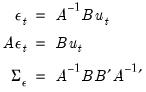 | (44.33) |
We may use the estimated moments

along with the

unique covariance equations in
Equation (44.33) to estimate the

elements in

and

. Satisfying the order condition requires an additional
restrictions for identification.
Restrictions on

and

take the form of assumptions about the structure of contemporaneous feedback of variables in the SVAR and assumptions about the correlation structure of the errors, respectively.
S Restrictions (Short-run)
The short-run S model is given by:
 | (44.34) |
We may use estimates

along with covariance restrictions in
Equation (44.34) to estimate the elements of

.
The S model may be more convenient to specify in that it involves the

element product

matrix and not the

elements in the individual

and

. Thus, the order condition only requires an additional

restrictions for identification.
This convenience comes at a cost, however, as the individual

and

matrices as the latter are not identified from

alone. For example, a given S model with

is equivalent to an A-B model with

and

, or an A-B model with

and

.
Thus, restrictions on

take the form of restrictions on the composite factor loadings, but offer no insight into the decomposition into endogeneity

and error loading components

.
F Restrictions (Long-run)
The identifying restrictions embodied in the relations

and

are commonly referred to as short-run restrictions. Blanchard and Quah (1989) proposed an alternative identification method using restrictions on the long-run properties of the accumulated impulse responses.
We may write these long-run restrictions as:
 | (44.35) |
where
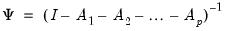
is the long-run multiplier, which may be estimated using the reduced form VAR parameter estimates. Note that the long-run F model is related to the S model through

and that as in the S model, the order condition requires an additional
restrictions.
The F model employs estimates of the moments

along with covariance relationships and restrictions from
Equation (44.32) to estimate the

elements in

. Thus, long-run identifying restrictions are specified in terms of the elements of this

matrix, typically in the form of zero restrictions. The restriction

means that the (accumulated) response of the
i-th variable to the
j-th structural shock is zero in the long-run.
Note that as with the S model, knowledge of

and

is sufficient to compute

, but the converse is not true.
Specifying SVAR Restrictions in EViews
EViews supports linear restrictions among the elements of matrices

,

,

, and

. In addition to commonly employed restrictions on single elements of the structural matrices, you may specify restrictions across elements of a given matrix, and you may even specify restrictions span

,

,

, and

.
For example, you may specify:
• a single element constant restriction,
e.g. 
• a general linear relationship within a single matrix,
e.g. 
or
• a general linear relationship that spans multiple matrices,
e.g. 
or
Restrictions in EViews are specified via pattern matrices and/or text expressions. Pattern matrices are a convenient way to place simple constant restrictions on individual elements of a structural matrix, while text expressions provide for the full range of supported restrictions.
A pattern matrix is a

matrix whose non-missing values,
i.e., non-NAs, specify constant restrictions on the corresponding matrix elements. All missing values,
i.e., NAs, place no restrictions on the corresponding matrix elements (such elements many still be restricted via text expressions). For example, suppose you want to restrict
A to be unit lower triangular and
B to be diagonal. With

the following pattern matrices could be employed:
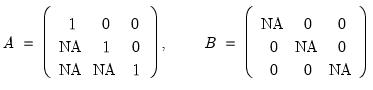 | (44.36) |
Text expressions allow you to write linear equations or use a function-like syntax to specify restrictions on one or more matrix elements. For example, replicating some of the earlier restrictions:
@a(1,1) = 2.5
@b(2,2) = @b(3,3) / 2
@a(1,1) + @a(2,1) = 1
@a(1,2) = 3 * @b(3,3)
@s(1,1) + @s(2,2) - @f(3,3) = 1.5
Notice that the EViews text syntax requires that the canonical structural matrix names are preceded by “@” to avoid ambiguity with workfile objects, e.g., scalars or matrix object elements.
In addition, EViews offers function-like expressions that concisely specify popular sets of restrictions. In the following list, the token

can be substituted with any of the canonical matrices

,

,

, and

. The canonical names should not be preceded by “@” in this context since there is no potential workfile object ambiguity in the function argument(s).
@X = mat | Use mat as a pattern matrix for matrix X, e.g., “@a=mat1”, “@b = @mat2”. |
| Restricts all elements of matrix X similar using the specified pattern matrix (provided in list form). Element ordering matches the vectorization of the matrix, i.e., the elements of the first column, followed by the second column, followed by the third column, etc. |
@diag(X) | Restricts X to be a diagonal matrix, i.e., off-diagonal elements are zero. The diagonal elements are unrestricted. |
@diag(X) = n | Restricts X to be a diagonal matrix with elements on the diagonal restricted to be n. |
@lower(X) | Restricts X to be a lower triangular matrix, i.e., elements above the diagonal are zero. |
@unitlower(X) | Restricts X to be a unit lower triangular matrix, i.e., elements above the diagonal are zero and elements on the diagonal are one. |
@upper(X) | Restricts X to be an upper triangular matrix, i.e., elements below the diagonal are zero. |
@unitupper(X) | Restricts X to be a unit upper triangular matrix, i.e., elements below the diagonal are zero and elements on the diagonal are one. |
@row(X, r) = n | Restricts the elements in row r of X to equal n. |
@col(X, c) = n | Restricts the elements in column c of X equal n. |
Examples
Suppose we wish to recreate a recursive Cholesky orthogonalization (using the order of the variables in the VAR specification). This restriction is equivalent to requiring that the

matrix is lower triangular. In the SVAR dialog (
“Restrictions”) there is for exactly this scenario, but we can also use a pattern matrix or text expression to restrict
S. For simplicity we’ll assume an underlying VAR named V1 with three endogenous variables (

). Each of the following sequences of commands produces the same set of S model restrictions and then estimates the model:
Approach #1: Using a pattern matrix
matrix(3, 3) pattern
pattern.fill na, na, na, 0, na, na, 0, 0, na
v1.svar(s=pattern)
Approach #2: Using a text expression equivalent to a pattern matrix
v1.append(svar) @vec(s) = na, na, na, 0, na, na, 0, 0, na
v1.svar
Approach #3: Using a text expression with specialized function
v1.append(svar) @lower(s)
v1.svar
For the next example, suppose we wish to estimate an A-B model where

captures only the standard deviations of the structural innovations so that the off-diagonal elements of

are set to zero. For

, these six restrictions fall short of the twelve restrictions necessary to satisfy the order condition, so (at least) six additional restrictions are required. To satisfy the order condition, we will restrict matrix

to have ones along the diagonal and require

,

, and

.
Approach #1: Using pattern matrices when possible
matrix(3, 3) patternA
patternA.fill 1, na, na, 0, 1, na, 0, na, 1
matrix(3, 3) patternB
patternB.fill na, 0, 0, 0, na, 0, 0, 0, na
v1.append(svar) @a(2,1) = @a(3,1)
v1.svar(a=patternA, b=patternB)
Approach #2: Using text expressions when possible
v1.append(svar) @vec(a) = 1, na, na, 0, 1, na, 0, na, 1
v1.append(svar) @a(2,1) = @a(3,1)
v1.append(svar) @diag(b)
v1.svar
Finally, suppose we wish to restrict the long-run impulse responses of an SVAR system. For illustrative purposes, suppose the responses of some variables to innovations are precisely half the responses of other variables, specifically
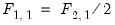
,
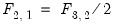
, and
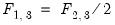
. Since these restrictions all involve more than one element

, we must use text expressions to specify the linear restrictions
v1.append(svar) @f(1,1) = @f(2,1) / 2
v1.append(svar) @f(2,1) = @f(3,2) / 2
v1.append(svar) @f(1,3) = @f(2,3) / 2
v1.svar
Estimating an SVAR in EViews
Once you have estimated a reduced form VAR, the SVAR specification and estimation dialog may be displayed by selecting You may use the dialog to specify a base collection of restrictions, customize restrictions on the four canonical matrices, and adjust options for the estimation procedure.
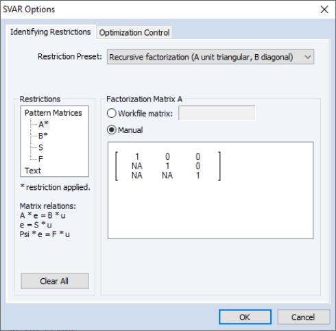
Restrictions
The tab allows you to specify your SVAR restrictions.
The drop-down menu provides a variety of pre-built restriction templates that can be applied to the SVAR model. Several of the presets can be used as is, while others require additional restrictions to meet the order condition.
The selection area on the left of the dialog allows you to view the current pattern matrices for any and all of the four canonical matrices as well as the current collection of text expression restrictions. Selecting a matrix element will change the dialog display to show the current restrictions for that matrix. There are two methods for specifying restrictions:
• Select and enter the elements directly in the dialog.
• Use the edit field to provide the name of a matrix in the workfile that contains the desired patterns.
To you click on the entry in the selection area, you may enter the specification of your restrictions using the syntax described above (
“Specifying SVAR Restrictions in EViews”).
Note that when a restriction has been applied to any of the selections, the left-hand side of the dialog will display the message “* restriction applied” and the names in the selection area will display a matching “*” as appropriate.
Lastly, we caution you that using the dropdown to select a preset will specify appropriate initial matrix restrictions, so that any existing customization will be overwritten.
Optimization
The log likelihood is maximized using Newton-Raphson with the Marquardt trust-region technique, analytic gradients, and numeric Hessians.
See “Marquardt”). See Amisano and Giannini (1997) for the analytic expression of the first derivatives.
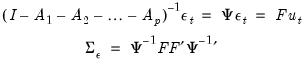
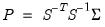
Estimation of the SVAR model is based on the relation

, with

specified in terms of elements of

and

, or

, or

, which in turn depend on

. We estimate

via maximum likelihood using the concentrated log-likelihood function:
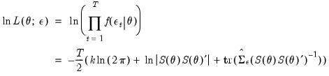 | (44.37) |
where

is the probability density function of the multivariate normal distribution with zero mean and

is the matrix trace operation.
As the underlying parameterization of the model in EViews involves a few idiosyncrasies, a few comments are in order:
• The underlying estimation parameters

will be used to form elements of

and

, or elements of
S, or elements of
F (mirroring the A-B, S, and F models), with the parameterization chosen to reflect the specified restrictions.
• EViews parametrically enforces your restrictions by analytically determining a set of unconstrained free parameters in one of the three above models. The models are prioritized, from highest to lowest: A-B, then S, and then F.
If, for example, the restrictions are in terms of a simple A-B model, then the parameterization will be in terms of the elements of

and

. If the restrictions are in terms of

and

, then the restrictions on

would be converted to restrictions on elements of

.
Regardless of which parameterization is used, the parameters can be used to calculate

and the likelihood.
In the special case of an A-B model with additional restrictions on

or

there is an additional complication, since restrictions on

or

cannot, in general, be converted to restrictions on

and

. In this setting, restrictions on

and

are enforced numerically through inclusion of a penalty term in the log-likelihood function.
As the penalty function approach does not actually reduce the number of parameters, this scenario produces a situation where the parameters may technically be under-identified. Ideally, the penalized log-likelihood function can guide the optimizer to convergence as if the extra parameters did not exist. However, convergence can be more difficult to achieve, even when the model is correctly identified. We therefore recommend that when using an A‑B model, the number of restrictions on

and

be kept to a minimum.
Once you provide identifying restrictions, you are ready to estimate the SVAR. Simply click on to estimate the model.
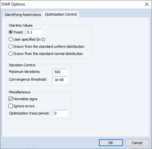
Prior to estimation, you may first to click on the Optimization Control tab in the SVAR Options dialog to show and modify the estimation settings:
There are three sets of settings for you to consider.
Starting Values
The starting values are those for the unconstrained parameters after substituting out the constraints.
Fixed sets all free parameters to the value specified in the edit field.
User Specified uses the values in the coefficient vector as specified in text form as starting values. For restrictions specified in pattern form, user specified starting values are taken from the first

elements of the default
C coefficient vector, where

is the number of free parameters. The
Draw from... options randomly draw the starting values for the free parameters from the specified distributions.
Iteration Control
Options for controlling the optimization process are provided in the Optimization Control tab of the SVAR Options dialog. You have the option to specify the maximum number of iterations, and the convergence criterion.
Sign Restrictions
For some restrictions, the signs of the matrices are not identified; see Christiano, Eichenbaum, and Evans (1999) for a discussion of this issue. When the sign is indeterminate, EViews will choose a post-estimation normalization such that the diagonal elements of matrix

are positive, with a further preference for the diagonal elements of matrix

to be positive in model. While it is not always possible to make the diagonal elements positive, this normalization procedure attempts to give all structural impulses positive signs (as well as the Cholesky factorization). The EViews default behavior applies this normalization rule whenever applicable. If you do not want to normalize the signs, deselect the option.
Ignore Errors
The checkbox instructs EViews to suppress “Near Singular Matrix” and other error messages during estimation. Consequently, if an error occurs, estimation results may be incomplete and inaccurate.
Optimization Trace
The tells EViews to summarize the ongoing optimization (iteration number, log-likelihood, parameter values) at the user-specified interval. Summary information is displayed in an unnamed text object.
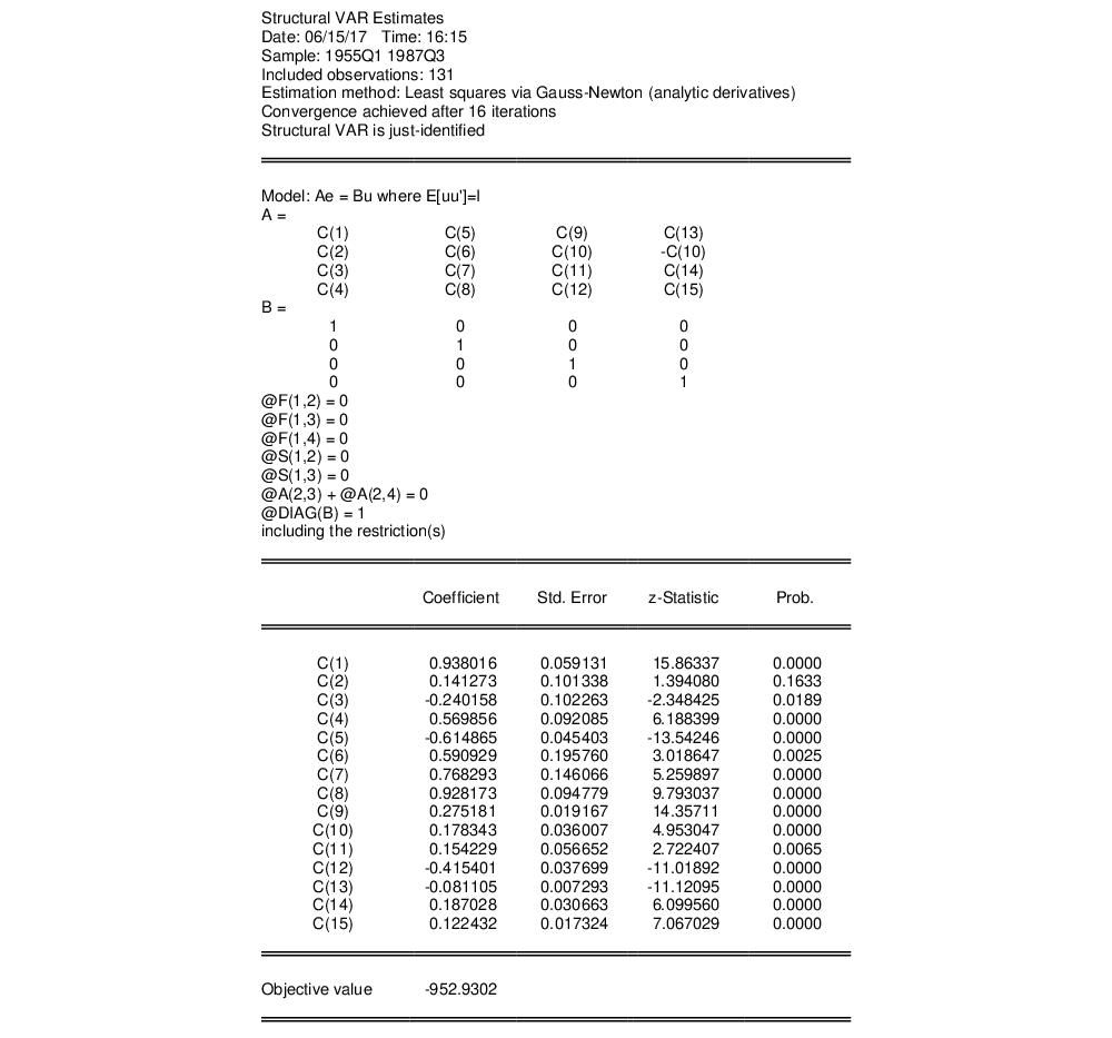
Estimation Output
Once optimization convergence is achieved, EViews displays the estimation output in the VAR window. The point estimates, standard errors, and z-statistics of the estimated free parameters are reported together with the maximized value of the log likelihood. The estimated standard errors are based on the inverse of the estimated information matrix (negative expected value of the Hessian) evaluated at the final parameter estimates.
For over-identified models, we also report the LR test for over-identification. The LR test statistic is computed as:
where
. Under the null hypothesis that the restrictions are valid, the LR statistic is asymptotically distributed as

, where

is the number of identifying restrictions.
The top portion of your SVAR output will show the restrictions, parameterization, and estimated coefficients,
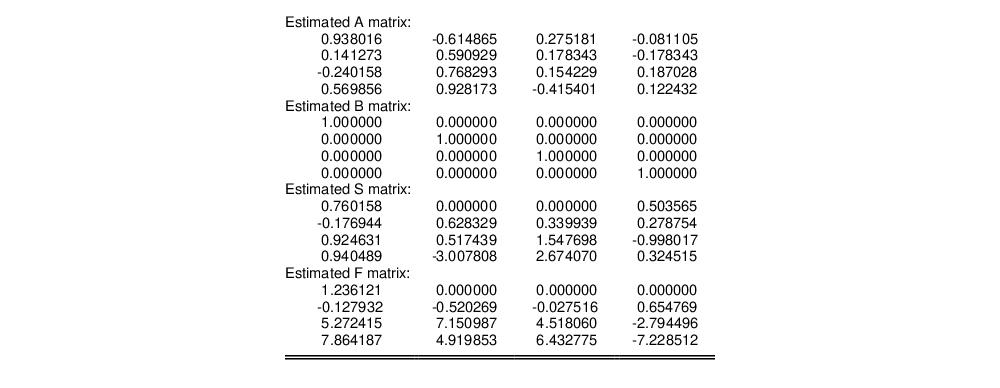
while the bottom portion shows the structural matrix estimates,
If you switch the view of the VAR window, you can come back to the previous results (without reestimating) by selecting from the VAR window. In addition, some of the SVAR estimation results can be retrieved as data members of the VAR; see
“Var Data Members” for a list of available VAR data members.
 ,
,  ,
,  , ...
, ...