Vector Autoregressions (VARs)
The vector autoregression (VAR) is commonly used for forecasting systems of interrelated time series and for analyzing the dynamic impact of random disturbances on the system of variables. The reduced form VAR approach sidesteps the need for structural modeling by treating every endogenous variable in the system as a function of p-lagged values of all of the endogenous variables in the system.
Below, we offer an abbreviated description of important features of the model. There are countless treatments of the basics of VAR analysis that one can consult for additional detail (see, for example, Lütkepohl, 2006).
We may write the stationary,

-dimensional, VAR(
p) process as
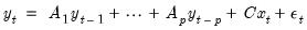 | (44.1) |
where
• 
is a

vector of endogenous variables,
• 
is a

vector of exogenous variables,
• 
are

matrices of lag coefficients to be estimated,
• 
is a

matrix of exogenous variable coefficients to be estimated,
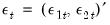
• 
is a

white noise innovation process, with

,
, and

for

.
The last statement implies that the vector of innovations are contemporaneously correlated with full rank matrix

, but are uncorrelated with their leads and lags of the innovations and (assuming the usual

orthogonality) uncorrelated with all of the right-hand side variables.
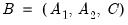
Let the

vector
 | (44.2) |
represent all of the period
t regressors in the VAR. Then for observations

, we may write this model in compact system form as:
 | (44.3) |
where
and
are

matrices of endogenous variables and innovations, and
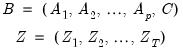 | (44.4) |
are the

matrix of system coefficients and the

matrix of regressor data, respectively.
In stacked form, we have
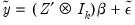 | (44.5) |
Since only lagged values of the endogenous variables appear on the right-hand side of the VAR equations
Equation (44.1) and the innovations are assumed to be uncorrelated with lagged innovations and the exogenous regressors, standard orthogonality conditions hold and OLS yields consistent estimates.
Furthermore, even though the innovations

may be contemporaneously correlated, all of the equations in the system have identical

regressors so that OLS is both equivalent to GLS and efficient. Accordingly, estimation of the standard VAR model in EViews is performed using simple OLS applied to each equation. (Later, when we describe estimation of restricted VAR models, we relax the identical regressors assumption so that OLS is no longer efficient.)
Applying least squares estimation to the stacked representation yields the least squares estimator
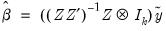 | (44.6) |
which has covariance matrix
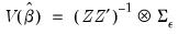 | (44.7) |
To obtain an estimator of the covariance matrix we require an estimate of

, which is typically obtained using the d.f. corrected residual moment estimator:
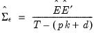 | (44.8) |
where

for

As an example, suppose that industrial production (IP) and money supply (M1) are jointly determined by a VAR(2) and let a constant be the only exogenous variable. Then the VAR may be written as:
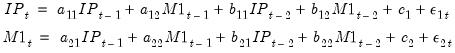 | (44.9) |
where

,

,

are the parameters to be estimated.
Alternately, in terms of
Equation (44.1), we have
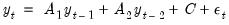 | (44.10) |
where

and
are

,

and

are

matrices, and

is

.
Further, we may write the specification in system or stacked form using
Equation (44.3),
Equation (44.4), and
Equation (44.5) with

and
.
Estimates of the coefficients of the VAR may be obtained by regressing IP on an intercept and two lags of IP and M1 and by regressing M1 on an intercept and two lags of IP and M1.
Estimating a VAR in EViews
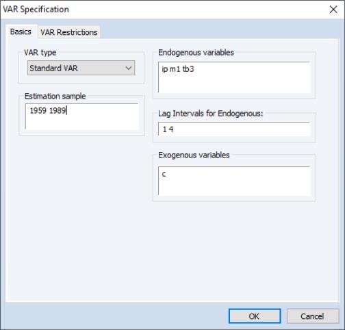
To specify a VAR in EViews, you must first create a Var object. Select or type var in the command window to display the estimation dialog
The Basics tab of the VAR Specification dialog will prompt you to define the structure of your VAR.
We begin with a simple reduced form VAR. You should fill out the dialog with the appropriate information:
• Select the VAR type: Standard VAR.
• Set the estimation sample.
• Enter a list of

in the corresponding edit field. You may list the series individually or you may include one or more series in a group object and enter the group name.
Here we have listed M1, IP, and TB3 as endogenous series
• Enter the lag specification in the edit box. This information is entered in pairs where each pair of numbers defines a range of lags. For example, the lag pair shown above:
1 4
tells EViews to use the first through fourth lags of all the endogenous variables in the system as right-hand side variables.
Through use of multiple lag pairs you may place zero restrictions on particular lag coefficient matrices

, as desired. Simply add any number of lag intervals, all entered in pairs, omitting those lags you wish to restrict. For example, he lag specification:
2 4 6 9 12 12
uses lags 2–4, 6–9, and 12.
Note that restrictions entered in this fashion restrict the entire

matrix to be zero. Below, we describe tools that allow for finer discrimination.
• Enter the specification for the exogenous series in the appropriate edit box, using group names if convenient.
Here, we have used the special series C to indicate that the VAR has a single constant exogenous term.
For the moment, we will ignore the VAR Restrictions tab of the dialog. Once you have specified your VAR, click on to have EViews estimate the coefficient matrices using least squares.
Estimation Output
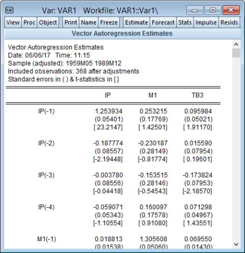
Following estimation, EViews will estimate the model EViews will display the estimation results in the VAR window.
Recall that our VAR specification has three (

) endogenous variables, IP, M1, and TB3, the exogenous intercept C (

), and includes lags 1 to 4 (

). Thus, there are (

) regressors in each of the three equations in the VAR.
As you can see, EViews displays the coefficient results in table. Each column in the table corresponds to an equation in the VAR, and each row corresponds to a regressor in the equation. Note that the regressors are grouped by variable, so that all of the lags for the first variable, here IP, are followed by all of the lags for the second variable, M1, and so on. The exogenous variables appear last.
For each right-hand side variable, EViews reports the estimated coefficient, its standard error, and the t-statistic. For example, the coefficient for IP(-1) in the TB3 equation is 0.095984, the standard error is 0.05021, and the corresponding t-statistic is 1.91170.
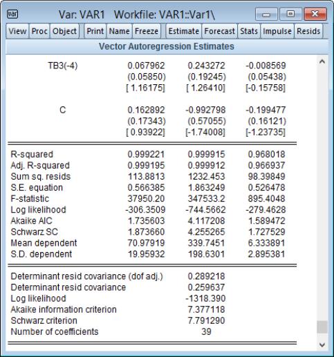
EViews displays additional information below the coefficient results. This information is divided into two parts:
• The first part of the additional output presents standard OLS regression summary statistics at the bottom of the column for the corresponding equation (recall that for the standard VAR each equation is estimated separately by OLS).
• The second part consists of summary statistics for the VAR system as a whole. These statistics include the determinant of the residual covariance, log-likelihood and associated information criteria, and number of coefficients:
A couple of comments on the calculation of the system statistics.
• The determinant of the residual covariance (degree-of-freedom adjusted) is computed as:
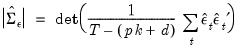 | (44.11) |
where you will recall that

is the number of parameters per equation in the VAR. The unadjusted calculation ignores the number of parameters and divides by

.
• The log likelihood value is computed assuming a multivariate normal (Gaussian) distribution as:
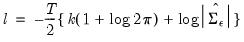 | (44.12) |
using the unadjusted determinant.
• The two information criteria are computed as:
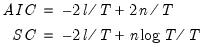 | (44.13) |
where
is the total number of estimated parameters in the VAR. The information criteria can be used for model selection such as determining the lag length of the VAR, with smaller values of the information criterion being preferred. Bear in mind when comparing the IC with other sources that some define the AIC/SC differently, either omitting the “inessential” constant terms from the likelihood, or by not dividing by

(see also
Appendix E. “Information Criteria” for additional discussion of information criteria).
 ,
,  , and
, and  , where
  .
.