Unit Root Testing
The theory behind ARMA estimation is based on stationary time series. A series is said to be (weakly or covariance) stationary if the mean and autocovariances of the series do not depend on time. Any series that is not stationary is said to be nonstationary.
A common example of a nonstationary series is the random walk:
 | (42.19) |
where
is a stationary random disturbance term. The series
has a constant forecast value, conditional on
, and the variance is increasing over time. The random walk is a difference stationary series since the first difference of
is stationary:
 | (42.20) |
A difference stationary series is said to be
integrated and is denoted as I(

) where

is the order of integration. The order of integration is the number of unit roots contained in the series, or the number of differencing operations it takes to make the series stationary. For the random walk above, there is one unit root, so it is an I(1) series. Similarly, a stationary series is I(0).
Standard inference procedures do not apply to regressions which contain an integrated dependent variable or integrated regressors. Therefore, it is important to check whether a series is stationary or not before using it in a regression. The formal method to test the stationarity of a series is the unit root test.
EViews provides you with a variety of powerful tools for testing a series (or the first or second difference of the series) for the presence of a unit root. In addition to Augmented Dickey-Fuller (1979) and Phillips-Perron (1988) tests, EViews allows you to compute the GLS-detrended Dickey-Fuller (Elliot, Rothenberg, and Stock, 1996), Kwiatkowski, Phillips, Schmidt, and Shin (KPSS, 1992), Elliott, Rothenberg, and Stock Point Optimal (ERS, 1996), and Ng and Perron (NP, 2001) unit root tests. All of these tests are available as a view of a series.
Performing Unit Root Tests in EViews
The following discussion assumes that you are familiar with the basic forms of the unit root tests and the associated options. We provide theoretical background for these tests in
“Basic Unit Root Theory”, and document the settings used when performing these tests.
To begin, double click on the series name to open the series window, and choose
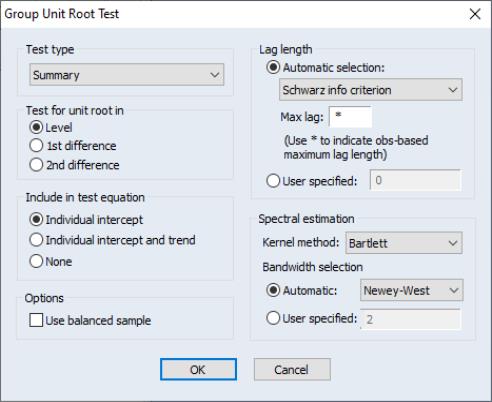
You must specify four sets of options to carry out a unit root test. The first three settings (on the left-hand side of the dialog) determine the basic form of the unit root test. The fourth set of options (on the right-hand side of the dialog) consist of test-specific advanced settings. You only need concern yourself with these settings if you wish to customize the calculation of your unit root test.
First, you should use the topmost dropdown menu to select the type of unit root test that you wish to perform. You may choose one of six tests: ADF, DFGLS, PP, KPSS, ERS, and NP.
Next, specify whether you wish to test for a unit root in the level, first difference, or second difference of the series.
Lastly, choose your exogenous regressors. You can choose to include a constant, a constant and linear trend, or neither (there are limitations on these choices for some of the tests).
You can click on OK to compute the test using the specified settings, or you can customize your test using the advanced settings portion of the dialog.
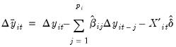
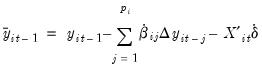
The advanced settings for both the ADF and DFGLS tests allow you to specify how lagged difference terms

are to be included in the ADF test equation. You may choose to let EViews automatically select

, or you may supply a fixed positive integer value. If you choose automatic selection, you will be given options for specifying both the lag selection method and maximum number of lags to be used in the selection procedure.
In this case, we have chosen to estimate an ADF test that includes a constant in the test regression and employs automatic lag length selection using a Schwarz Information Criterion (BIC) and a maximum lag length of 14. Applying these settings to data on the U.S. one-month Treasury bill rate for the period from March 1953 to July 1971 (“Hayashi_92.WF1”), we can replicate Example 9.2 of Hayashi (2000, p. 596). The results are described below.
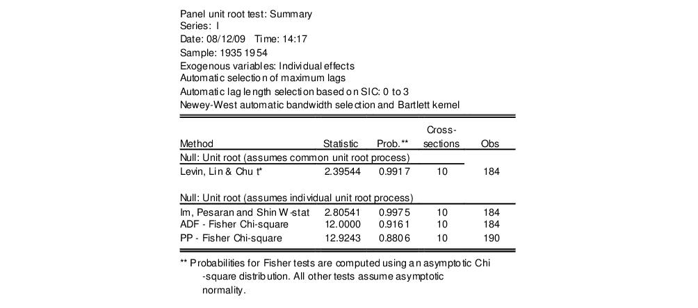
The first part of the unit root output provides information about the form of the test (the type of test, the exogenous variables, and lag length used), and contains the test output, associated critical values, and in this case, the p-value:
The ADF statistic value is -1.417 and the associated one-sided
p-value (for a test with 221 observations) is .573. In addition, EViews reports the critical values at the 1%, 5% and 10% levels. Notice here that the statistic

value is greater than the critical values so that we do not reject the null at conventional test sizes.
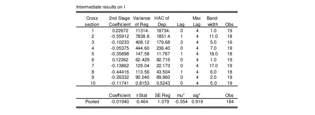
The second part of the output shows the intermediate test equation that EViews used to calculate the ADF statistic:
If you had chosen to perform any of the other unit root tests (PP, KPSS, ERS, NP), the right side of the dialog would show the different options associated with the specified test. The options are associated with the method used to estimate the zero frequency spectrum term,

, that is used in constructing the particular test statistic. As before, you only need pay attention to these settings if you wish to change from the EViews defaults.
Here, we have selected the PP test in the dropdown menu. Note that the right-hand side of the dialog has changed, and now features a dropdown menu for selecting the spectral estimation method. You may use this dropdown menu to choose between various kernel or AR regression based estimators for

. The entry labeled “Default” will show you the default estimator for the specific unit root test—in this example, we see that the PP default uses a kernel sum-of-covariances estimator with Bartlett weights. Alternately, if you had selected a NP test, the default entry would be “AR spectral-GLS”.
Lastly, you can control the lag length or bandwidth used for your spectral estimator. If you select one of the kernel estimation methods (Bartlett, Parzen, Quadratic Spectral), the dialog will give you a choice between using Newey-West or Andrews automatic bandwidth selection methods, or providing a user specified bandwidth. If you choose one of the AR spectral density estimation methods (AR Spectral - OLS, AR Spectral - OLS detrended, AR Spectral - GLS detrended), the dialog will prompt you to choose from various automatic lag length selection methods (using information criteria) or to provide a user-specified lag length. See
“Automatic Bandwidth and Lag Length Selection”.
Once you have chosen the appropriate settings for your test, click on the
OK button. EViews reports the test statistic along with output from the corresponding test regression. For these tests, EViews reports the uncorrected estimate of the residual variance and the estimate of the frequency zero spectrum

(labeled as the “HAC corrected variance”) in addition to the basic output. Running a PP test using the TBILL series using the Andrews bandwidth yields:
As with the ADF test, we fail to reject the null hypothesis of a unit root in the TBILL series at conventional significance levels.
Note that your test output will differ somewhat for alternative test specifications. For example, the KPSS output only provides the asymptotic critical values tabulated by KPSS:
Similarly, the NP test output will contain results for all four test statistics, along with the NP tabulated critical values.
A word of caution. You should note that the critical values reported by EViews are valid only for unit root tests of a data series, and will be invalid if the series is based on estimated values. For example, Engle and Granger (1987) proposed a two-step method of testing for cointegration which looks for a unit root in the residuals of a first-stage regression. Since these residuals are estimates of the disturbance term, the asymptotic distribution of the test statistic differs from the one for ordinary series. See
“Cointegration Testing” for EViews routines to perform testing in this setting.
Basic Unit Root Theory
The following discussion outlines the basics features of unit root tests. By necessity, the discussion will be brief. Users who require detail should consult the original sources and standard references (see, for example, Davidson and MacKinnon, 1993, Chapter 20, Hamilton, 1994, Chapter 17, and Hayashi, 2000, Chapter 9).
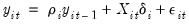
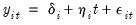
Consider a simple AR(1) process:
 | (42.21) |
where

are optional exogenous regressors which may consist of constant, or a constant and trend,

and

are parameters to be estimated, and the

are assumed to be white noise. If

,

is a nonstationary series and the variance of

increases with time and approaches infinity. If

,

is a (trend-)stationary series. Thus, the hypothesis of (trend-)stationarity can be evaluated by testing whether the absolute value of

is strictly less than one.
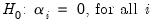
The unit root tests that EViews provides generally test the null hypothesis

against the one-sided alternative

. In some cases, the null is tested against a point alternative. In contrast, the KPSS Lagrange Multiplier test evaluates the null of

against the alternative

.
The Augmented Dickey-Fuller (ADF) Test
The standard DF test is carried out by estimating
Equation (42.21) after subtracting
from both sides of the equation:
 | (42.22) |
where
. The null and alternative hypotheses may be written as,
 | (42.23) |
and evaluated using the conventional

-ratio for
:
 | (42.24) |
where

is the estimate of
, and

is the coefficient standard error.
Dickey and Fuller (1979) show that under the null hypothesis of a unit root, this statistic does not follow the conventional Student’s
t-distribution, and they derive asymptotic results and simulate critical values for various test and sample sizes. More recently, MacKinnon (1991, 1996) implements a much larger set of simulations than those tabulated by Dickey and Fuller. In addition, MacKinnon estimates response surfaces for the simulation results, permitting the calculation of Dickey-Fuller critical values and
-values for arbitrary sample sizes. The more recent MacKinnon critical value calculations are used by EViews in constructing test output.
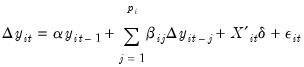
The simple Dickey-Fuller unit root test described above is valid only if the series is an AR(1) process. If the series is correlated at higher order lags, the assumption of white noise disturbances

is violated. The Augmented Dickey-Fuller (ADF) test constructs a parametric correction for higher-order correlation by assuming that the

series follows an AR(

) process and adding

lagged difference terms of the dependent variable

to the right-hand side of the test regression:
 | (42.25) |
This augmented specification is then used to test
(42.23) using the
-ratio
(42.24). An important result obtained by Fuller is that the asymptotic distribution of the

-ratio for

is independent of the number of lagged first differences included in the ADF regression. Moreover, while the assumption that

follows an autoregressive (AR) process may seem restrictive, Said and Dickey (1984) demonstrate that the ADF test is asymptotically valid in the presence of a moving average (MA) component, provided that sufficient lagged difference terms are included in the test regression.
You will face two practical issues in performing an ADF test. First, you must choose whether to include exogenous variables in the test regression. You have the choice of including a constant, a constant and a linear time trend, or neither in the test regression. One approach would be to run the test with both a constant and a linear trend since the other two cases are just special cases of this more general specification. However, including irrelevant regressors in the regression will reduce the power of the test to reject the null of a unit root. The standard recommendation is to choose a specification that is a plausible description of the data under both the null and alternative hypotheses. See Hamilton (1994, p. 501) for discussion.
Second, you will have to specify the number of lagged difference terms (which we will term the “lag length”) to be added to the test regression (0 yields the standard DF test; integers greater than 0 correspond to ADF tests). The usual (though not particularly useful) advice is to include a number of lags sufficient to remove serial correlation in the residuals. EViews provides both automatic and manual lag length selection options. For details, see
“Automatic Bandwidth and Lag Length Selection”.
Dickey-Fuller Test with GLS Detrending (DFGLS)
As noted above, you may elect to include a constant, or a constant and a linear time trend, in your ADF test regression. For these two cases, ERS (1996) propose a simple modification of the ADF tests in which the data are detrended so that explanatory variables are “taken out” of the data prior to running the test regression.
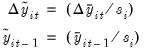
ERS define a quasi-difference of

that depends on the value

representing the specific point alternative against which we wish to test the null:
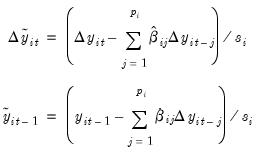 | (42.26) |
Next, consider an OLS regression of the quasi-differenced data

on the quasi-differenced

:
 | (42.27) |
where
contains either a constant, or a constant and trend, and let

be the OLS estimates from this regression.
All that we need now is a value for
. ERS recommend the use of

, where:
 | (42.28) |
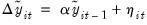
We now define the
GLS detrended data, 
using the estimates associated with the
:
 | (42.29) |
Then the DFGLS test involves estimating the standard ADF test equation,
(42.25), after substituting the GLS detrended
for the original
 :
: | (42.30) |
Note that since the

are detrended, we do not include the
in the DFGLS test equation. As with the ADF test, we consider the

-ratio for

from this test equation.
While the DFGLS
-ratio follows a Dickey-Fuller distribution in the constant only case, the asymptotic distribution differs when you include both a constant and trend. ERS (1996, Table 1, p. 825) simulate the critical values of the test statistic in this latter setting for
. Thus, the EViews lower tail critical values use the MacKinnon simulations for the no constant case, but are interpolated from the ERS simulated values for the constant and trend case. The null hypothesis is rejected for values that fall below these critical values.
The Phillips-Perron (PP) Test
Phillips and Perron (1988) propose an alternative (nonparametric) method of controlling for serial correlation when testing for a unit root. The PP method estimates the non-augmented DF test equation
(42.22), and modifies the

-ratio of the

coefficient so that serial correlation does not affect the asymptotic distribution of the test statistic. The PP test is based on the statistic:
 | (42.31) |
where

is the estimate, and

the
-ratio of

,

is coefficient standard error, and

is the standard error of the test regression. In addition,

is a consistent estimate of the error variance in
(42.22) (calculated as

, where

is the number of regressors). The remaining term,
, is an estimator of the residual spectrum at frequency zero.
There are two choices you will have make when performing the PP test. First, you must choose whether to include a constant, a constant and a linear time trend, or neither, in the test regression. Second, you will have to choose a method for estimating
. EViews supports estimators for

based on kernel-based sum-of-covariances, or on autoregressive spectral density estimation. See
“Frequency Zero Spectrum Estimation” for details.
The asymptotic distribution of the PP modified

-ratio is the same as that of the ADF statistic. EViews reports MacKinnon lower-tail critical and
p-values for this test.
The Kwiatkowski, Phillips, Schmidt, and Shin (KPSS) Test
The KPSS (1992) test differs from the other unit root tests described here in that the series

is assumed to be (trend-) stationary under the null. The KPSS statistic is based on the residuals from the OLS regression of
on the exogenous variables

:
 | (42.32) |
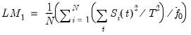
The LM statistic is be defined as:
 | (42.33) |
where

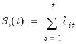
, is an estimator of the residual spectrum at frequency zero and where

is a cumulative residual function:
 | (42.34) |
based on the residuals
. We point out that the estimator of

used in this calculation differs from the estimator for

used by GLS detrending since it is based on a regression involving the original data and not on the quasi-differenced data.
To specify the KPSS test, you must specify the set of exogenous regressors

and a method for estimating

. See
“Frequency Zero Spectrum Estimation” for discussion.
The reported critical values for the LM test statistic are based upon the asymptotic results presented in KPSS (Table 1, p. 166).
Elliot, Rothenberg, and Stock Point Optimal (ERS) Test
The ERS Point Optimal test is based on the quasi-differencing regression defined in Equations
(42.27). Define the residuals from
(42.27) as

, and let

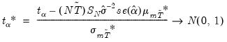
be the sum-of-squared residuals function. The ERS (feasible) point optimal test statistic of the null that

against the alternative that
, is then defined as:
 | (42.35) |
where

, is an estimator of the residual spectrum at frequency zero.
To compute the ERS test, you must specify the set of exogenous regressors

and a method for estimating

(see
“Frequency Zero Spectrum Estimation”).
Critical values for the ERS test statistic are computed by interpolating the simulation results provided by ERS (1996, Table 1, p. 825) for

.
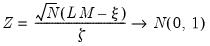
Ng and Perron (NP) Tests
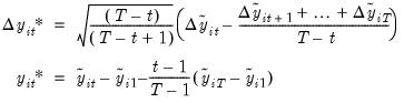
Ng and Perron (2001) construct four test statistics that are based upon the GLS detrended data

. These test statistics are modified forms of Phillips and Perron

and

statistics, the Bhargava (1986)

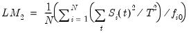
statistic, and the ERS Point Optimal statistic. First, define the term:
 | (42.36) |
The modified statistics may then be written as,
 | (42.37) |
where:
 | (42.38) |
The NP tests require a specification for

and a choice of method for estimating

(see
“Frequency Zero Spectrum Estimation”).
Frequency Zero Spectrum Estimation
Many of the unit root tests described above require a consistent estimate of the residual spectrum at frequency zero. EViews supports two classes of estimators for

: kernel-based sum-of-covariances estimators, and autoregressive spectral density estimators.
Kernel Sum-of-Covariances Estimation
The kernel-based estimator of the frequency zero spectrum is based on a weighted sum of the autocovariances, with the weights are defined by a kernel function. The estimator takes the form,
 | (42.39) |
where

is a bandwidth parameter (which acts as a truncation lag in the covariance weighting),

is a kernel function, and where

, the
j-th sample autocovariance of the residuals

, is defined as:
 | (42.40) |
Note that the residuals

that EViews uses in estimating the autocovariance functions in
(42.40) will differ depending on the specified unit root test:
| |
ADF, DFGLS | not applicable. |
PP, ERS Point Optimal, NP | residuals from the Dickey-Fuller test equation,
(42.22). |
KPSS | residuals from the OLS test equation,
(42.32). |
EViews supports the following kernel functions:
The properties of these kernels are described in Andrews (1991).
As with most kernel estimators, the choice of the bandwidth parameter

is of considerable importance. EViews allows you to specify a fixed parameter or to have EViews select one using a data-dependent method. Automatic bandwidth parameter selection is discussed in
“Automatic Bandwidth and Lag Length Selection”.
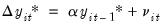
Autoregressive Spectral Density Estimator
The autoregressive spectral density estimator at frequency zero is based upon the residual variance and estimated coefficients from the auxiliary regression:
 | (42.41) |
EViews provides three autoregressive spectral methods: OLS, OLS detrending, and GLS detrending, corresponding to difference choices for the data

. The following table summarizes the auxiliary equation estimated by the various AR spectral density estimators:
| |
OLS | |
OLS detrended |  , and  . |
GLS detrended |  . and  . |
where

are the coefficient estimates from the regression defined in
(42.27).
The AR spectral estimator of the frequency zero spectrum is defined as:
 | (42.42) |
where

is the residual variance, and

are the estimates from
(42.41). We note here that EViews uses the non-degree of freedom estimator of the residual variance. As a result, spectral estimates computed in EViews may differ slightly from those obtained from other sources.
Not surprisingly, the spectrum estimator is sensitive to the number of lagged difference terms in the auxiliary equation. You may either specify a fixed parameter or have EViews automatically select one based on an information criterion. Automatic lag length selection is examined in
“Automatic Bandwidth and Lag Length Selection”.
Default Settings
By default, EViews will choose the estimator of

used by the authors of a given test specification. You may, of course, override the default settings and choose from either family of estimation methods. The default settings are listed below:
| |
ADF, DFGLS | not applicable |
PP, KPSS | Kernel (Bartlett) sum-of-covariances |
ERS Point Optimal | AR spectral regression (OLS) |
NP | AR spectral regression (GLS-detrended) |
Automatic Bandwidth and Lag Length Selection
There are three distinct situations in which EViews can automatically compute a bandwidth or a lag length parameter.
The first situation occurs when you are selecting the bandwidth parameter

for the kernel-based estimators of

. For the kernel estimators, EViews provides you with the option of using the Newey-West (1994) or the Andrews (1991) data-based automatic bandwidth parameter methods. See the original sources for details. For those familiar with the Newey-West procedure, we note that EViews uses the lag selection parameter formulae given in the corresponding first lines of Table II-C. The Andrews method is based on an AR(1) specification. (See
“Automatic Bandwidth Selection” for discussion.)
The latter two situations occur when the unit root test requires estimation of a regression with a parametric correction for serial correlation as in the ADF and DFGLS test equation regressions, and in the AR spectral estimator for

. In all of these cases,

lagged difference terms are added to a regression equation. The automatic selection methods choose

(less than the specified maximum) to minimize one of the following criteria:
| |
Akaike (AIC) | |
Schwarz (SIC) | |
Hannan-Quinn (HQ) | |
Modified AIC (MAIC) | |
Modified SIC (MSIC) | |
Modified Hannan-Quinn (MHQ) | |
where the modification factor

is computed as:
 | (42.43) |
for

, when computing the ADF test equation, and for

as defined in
“Autoregressive Spectral Density Estimator”, when estimating

. Ng and Perron (2001) propose and examine the modified criteria, concluding with a recommendation of the MAIC.
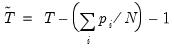
For the information criterion selection methods, you must also specify an upper bound to the lag length. By default, EViews chooses a maximum lag of:
 | (42.44) |
See Hayashi (2000, p. 594) for a discussion of the selection of this upper bound.


 residuals for kernel estimator


 , and
, and  ,
,  .
.


