EViews Help: Working with ARCH Models

Once your model has been estimated, EViews provides a variety of views and procedures for inference and diagnostic checking.

• The Representations view displays the estimation command as well as the estimation and substituted coefficients equations for the mean and variance specifications.

• The Actual, Fitted, Residual view displays the residuals in various forms, such as table, graphs, and standardized residuals. You can save the residuals as a named series in your workfile using a procedure (see “ARCH Model Procedures”).

• GARCH Graph/Conditional Standard Deviation and GARCH Graph/Conditional Variance plots the one-step ahead standard deviation

or variance

for each observation in the sample. The observation at period

is the forecast for

made using information available in

. You can save the conditional standard deviations or variances as named series in your workfile using a procedure (see below). If the specification is for a component model, EViews will also display the permanent and transitory components.

• Covariance Matrix displays the estimated coefficient covariance matrix. Most ARCH models (except ARCH-M models) are block diagonal so that the covariance between the mean coefficients and the variance coefficients is very close to zero. If you include a constant in the mean equation, there will be two C’s in the covariance matrix; the first C is the constant of the mean equation, and the second C is the constant of the variance equation.

• Coefficient Diagnostics produces standard diagnostics (confidence intervals and ellipses, Wald tests, omitted and redundant variables tests), for the estimated coefficients. See “Coefficient Diagnostics” for details. Note that the likelihood ratio tests are not appropriate under a quasi-maximum likelihood interpretation of your results.

• Coefficient Diagnostics/Nyblom Stability Test is a test of parameter stability or structural change. The test provides individual statistics on each parameter (both in the mean and variance equations) and a joint test of null hypothesis is that the parameters are constant through time.

• Residual Diagnostics/Correlogram–Q-statistics displays the correlogram (autocorrelations and partial autocorrelations) of the standardized residuals. This view can be used to test for remaining serial correlation in the mean equation and to check the specification of the mean equation. If the mean equation is correctly specified, all Q-statistics should not be significant. See “Correlogram” for an explanation of correlograms and Q-statistics.

• Residual Diagnostics/Correlogram Squared Residuals displays the correlogram (autocorrelations and partial autocorrelations) of the squared standardized residuals. This view can be used to test for remaining ARCH in the variance equation and to check the specification of the variance equation. If the variance equation is correctly specified, all Q-statistics should not be significant. See “Correlogram” for an explanation of correlograms and Q-statistics. See also Residual Diagnostics/ARCH LM Test.

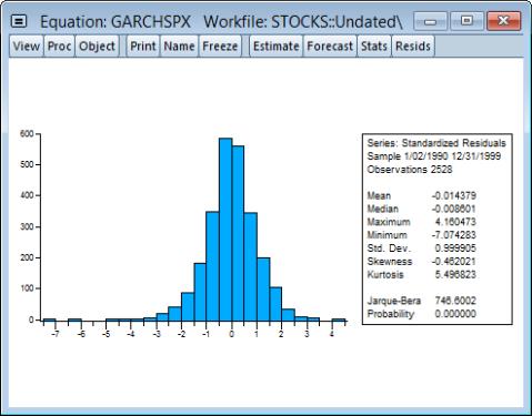
• Residual Diagnostics/Histogram–Normality Test displays descriptive statistics and a histogram of the standardized residuals. You can use the Jarque-Bera statistic to test the null of whether the standardized residuals are normally distributed. If the standardized residuals are normally distributed, the Jarque-Bera statistic should not be significant. See “Descriptive Statistics & Tests” for an explanation of the Jarque-Bera test. For example, the histogram of the standardized residuals from the GARCH(1,1) model fit to the daily stock return looks as follows:

The standardized residuals are leptokurtic and the Jarque-Bera statistic strongly rejects the hypothesis of normal distribution.

• Residual Diagnostics/ARCH LM Test carries out Lagrange multiplier tests to test whether the standardized residuals exhibit additional ARCH. If the variance equation is correctly specified, there should be no ARCH left in the standardized residuals. See “ARCH LM Test” for a discussion of testing. See also Residual Diagnostics/Correlogram Squared Residuals.

• Residual Diagnostics/Sign-Bias Test (Engle and Ng, 1993) provides a test for misspecification of the conditional variance model. The test performs a regression of the squared residuals against dummy variables based upon the sign previous residuals. If a GARCH model is correctly specified, the sign of previous residuals should have no impact upon the current squared residuals. The null hypothesis is that the parameters of the regression are zero.

Various ARCH equation procedures allow you to produce results based on you estimated equation. Some of these procedures, for example the Make Gradient Group and Make Derivative Group behave the same as in other equations. Some of the procedures have ARCH specific elements:

• Forecast uses the estimated ARCH model to compute static and dynamic forecasts of the mean, its forecast standard error, and the conditional variance. To save any of these forecasts in your workfile, type a name in the corresponding dialog box. If you choose the Forecast Graph option, EViews displays the graphs of the forecasts and two standard deviation bands for the mean forecast.

Note that the squared residuals

may not be available for presample values or when computing dynamic forecasts. In such cases, EViews will replaced the term by its expected value. In the simple GARCH(p, q) case, for example, the expected value of the squared residual is the fitted variance, e.g.,

. In other models, the expected value of the residual term will differ depending on the distribution and, in some cases, the estimated parameters of the model.

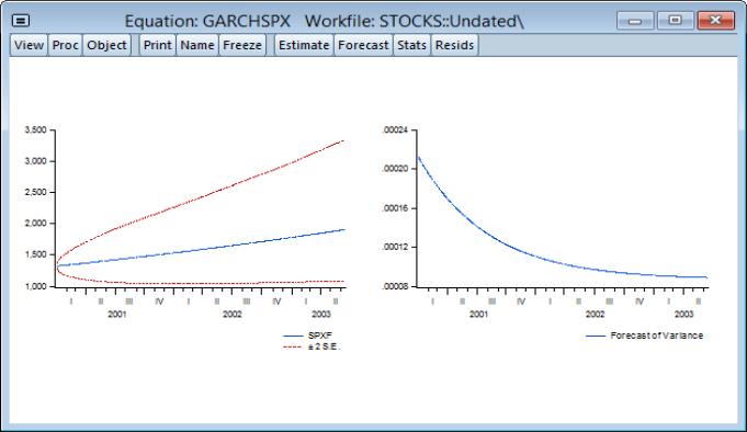
For example, to construct dynamic forecasts of SPX using the previously estimated model, click on Forecast and fill in the Forecast dialog, setting the sample to “2001m01 @last” so the dynamic forecast begins immediately following the estimation period. Unselect the Forecast Evaluation checkbox and click on OK to display the forecast results.

It will be useful to display these results in two columns. Right-mouse click then select Position and align graphs..., enter “2” for the number of Columns, and select Automatic spacing. Click on OK to display the rearranged graph:

The first graph is the forecast of SPX (SPXF) from the mean equation with two standard deviation bands. The second graph is the forecast of the conditional variance

• Make Residual Series saves the residuals as named series in your workfile. You have the option to save the ordinary residuals,

, or the standardized residuals,

. The residuals will be named RESID1, RESID2, and so on; you can rename the series with the name button in the series window.

• Make GARCH Variance Series... saves the conditional variances

as named series in your workfile. You should provide a name for the target conditional variance series and, if relevant, you may provide a name for the permanent component series. You may take the square root of the conditional variance series to get the conditional standard deviations as displayed by the View/GARCH Graph/Conditional Standard Deviation.