Examples
In this section, we offer three examples illustrating GLM estimation in EViews.
Exponential Regression
Our first example uses the Kennen (1983) dataset (“Strike.WF1”) on number of strikes (NUMB), industrial production (IP), and dummy variable representing the month of February (FEB). To account for the non-negative response variable NUMB, we may estimate a nonlinear specification of the form:
 | (32.3) |
where

. This model falls into the GLM framework with a log link and normal family. To estimate this specification, bring up the GLM dialog and fill out the equation specification page as follows:
numb c ip feb
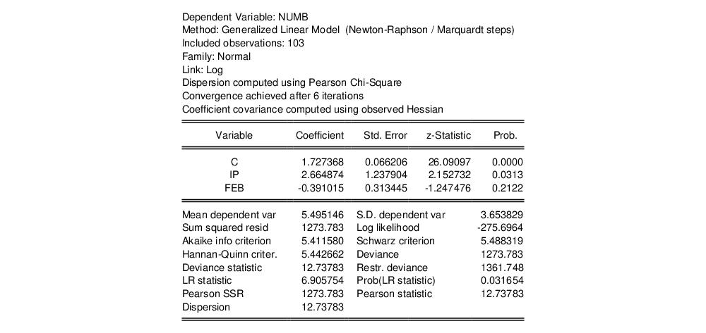
then change the to . For the moment, we leave the remaining settings and those on the page at their default values. Click on to accept the specification and estimate the model. EViews displays the following results:
The top portion of the output displays the estimation settings and basic results, in particular the choice of algorithm (Newton-Raphson with Marquardt steps), distribution family (Normal), and link function (Log), as well as the dispersion estimator, coefficient covariance estimator, and estimation status. We see that the dispersion estimator is based on the Pearson

statistic and the coefficient covariance is computed using the inverse of the (negative of the) observed Hessian.
The coefficient estimates indicate that IP is positively related to the number of strikes, and that the relationship is statistically significant at conventional levels. The FEB dummy variable is negatively related to NUMB, but the relationship is not statistically significant.
The bottom portion of the output displays various descriptive statistics. Note that in place of some of the more familiar statistics, EViews reports the deviance, deviance statistic (deviance divided by the degrees-of-freedom) restricted deviance (for the model with only a constant), and the corresponding LR test statistic and probability. The test indicates that the IP and FEB variables are jointly significant at roughly the 3% level. Also displayed are the sum-of-squared Pearson residuals and the estimate of the dispersion, which in this example is the Pearson statistic.
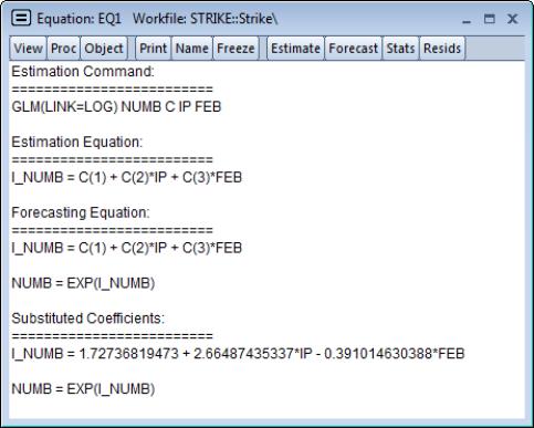
It may be instructive to examine the representations view of this equation. Simply go to the equation toolbar or the main menu and click on to display the view.
Notably, the representations view displays both the specification of the linear predictor (I_NUMB) as well as the mean specification (EXP(I_NUMB)) in terms of the EViews coefficient names, and in terms of the estimated values. These are the expressions used when forecasting the index or the dependent variable using the procedure (see
“Forecasting”).
Binomial
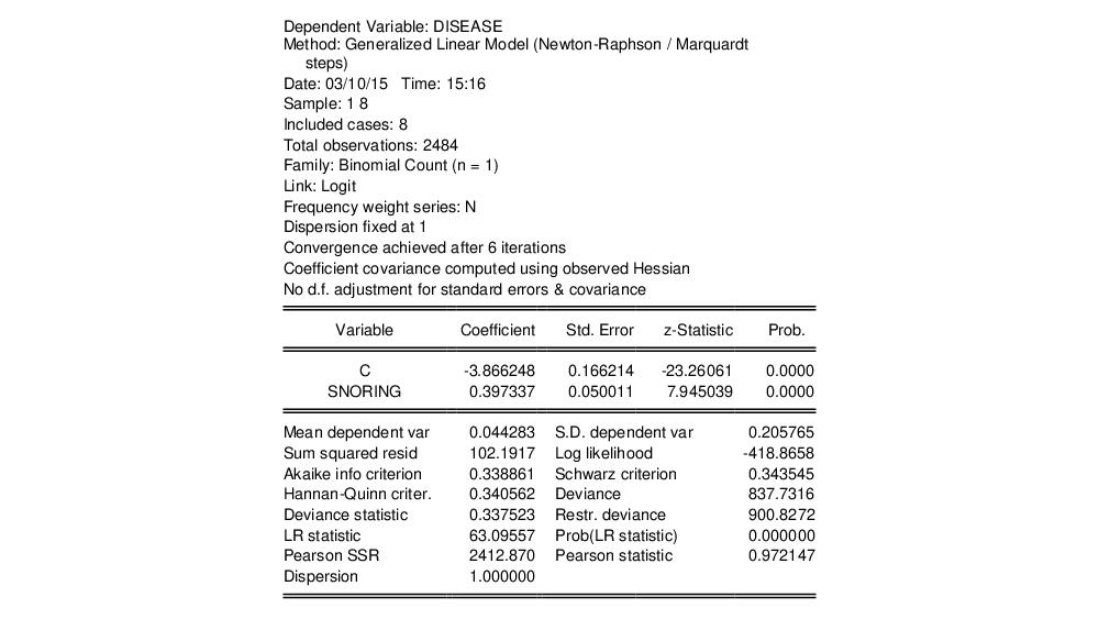
We illustrate the estimation of GLM binomial logistic regression using a simple example from Agresti (2007, Table 3.1, p. 69) examining the relationship between snoring and heart disease. The data in the first page of the workfile “Snoring.WF1” consist of grouped binomial response data for 2,484 subjects divided into four risk factor groups for snoring level (SNORING), coded as 0, 2, 4, 5. Associated with each of the four groups is the number of individuals in the group exhibiting heart disease (DISEASE) as well as a total group size (TOTAL).
We may estimate a logistic regression model for these data in either raw frequency or proportions form.
To estimate the model in raw frequency form, bring up the GLM equation dialog, enter the linear predictor specification:
disease c snore
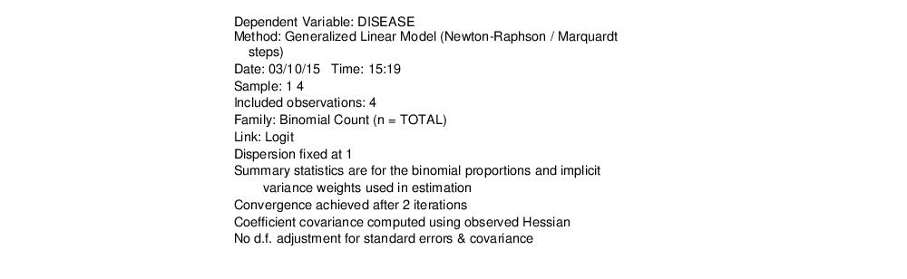
select in the dropdown, and enter “TOTAL” in the edit field. Next switch over to the page and turn off the for the coefficient covariance. Click on to estimate the equation.
The output header shows relevant information for the estimation procedure. Note in particular the EViews message that summary statistics are computed for the binomial proportions data. This message is a hint at the fact that EViews estimates the binomial count model by scaling the dependent variable by the number of trials, and estimating the corresponding proportions specification.
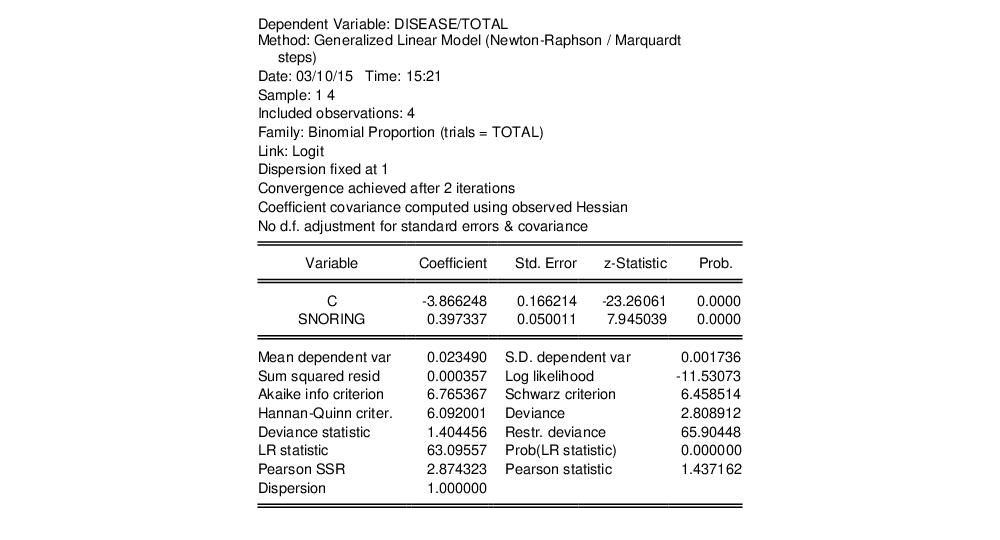
Accordingly, you could have specified the model in proportions form. Simply enter the linear predictor specification:
disease/total c snoring
with specified in the dropdown and “TOTAL” entered in the edit field.
The top portion of the output changes to show the different settings, but the remaining output is identical. In particular, there is strong evidence that SNORING is related to heart disease in these data, with the estimated probability of heart disease increasing with the level of snoring.
It is worth mentioning that data of this form are sometimes represented in a frequency weighted form in which the data each group is divided into two records, one for the binomial successes, and one for the failures. Each each record contains the number of repeats in the group and a binary indicator for success (the total number of records is

, where

is the number of groups) The FREQ page of the “Snoring.WF1” workfile contains the data represented in this fashion:
In this representation, DISEASE is an indicator for whether the record corresponds to individuals with heart disease or not, and N is the number of individuals in the category.
Estimation of the equivalent GLM model specified using the frequency weighted data is straightforward. Simply enter the linear predictor specification:
disease c snoring
with either or specified in the dropdown. Since each observation corresponds to a binary indicator, you should enter “1” enter as the edit field. The multiple individuals in the category are handled by entering “N” in the field in the page.
Note that while a number of the summary statistics differ due to the different representation of the data (notably the Deviance and Pearson SSRs), the coefficient estimates and LR test statistics in this case are identical to those outlined above. There will, however, be substantive differences between the two results in settings when the dispersion is estimated since the effective number of observations differs in the two settings.
Lastly the data may be represented in individual trial form, which expands observations for each trial in the group into a separate record. The total number of records in the data is

, where

is the number of trials in the
i-th (of

) group. This representation is the traditional ungrouped binary response form for the data. Results for data in this representation should match those for the frequency weighted data.
Binomial Proportions
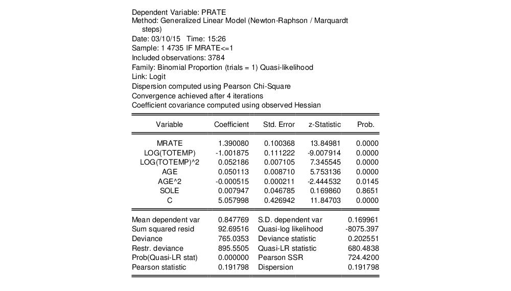
Papke and Wooldridge (1996) apply GLM techniques to the analysis of fractional response data for 401K tax advantaged savings plan participation rates (“401kjae.WF1”). Their analysis focuses on the relationship between plan participation rates (PRATE) and the employer matching contribution rates (MRATE), accounting for the log of total employment (LOG(TOTEMP), LOG(TOTEMP)^2), plan age (AGE, AGE^2), and a binary indicator for whether the plan is the only pension plan offered by the plan sponsor (SOLE).
We focus on two of the equations estimated in the paper. In both, the authors employ a GLM specification using a binomial proportion family and logit link. Information on the binomial group size

is ignored, but variance misspecification is accounted for in two ways: first using a binomial QMLE with GLM standard errors, and second using the robust Huber-White covariance approach.
To estimate the GLM standard error specification, we first call up the GLM dialog and enter the linear predictor specification:
prate mprate log(totemp) log(totemp)^2 age age^2 sole
Next, select the family, and enter the sample description
@all if mrate<=1
Lastly, we leave the edit field at the default value of 1, but correct for heterogeneity by going to the page and specifying dispersion estimates. Click on to continue.
The resulting estimates correspond the coefficient estimates and first set of standard errors in Papke and Wooldridge (Table II, column 2):
Papke and Wooldridge offer a detailed analysis of the results (p. 628–629), which we will not duplicate here. We will point out that the estimate of the dispersion (0.191798) taken from the Pearson statistic is far from the restricted value of 1.0.
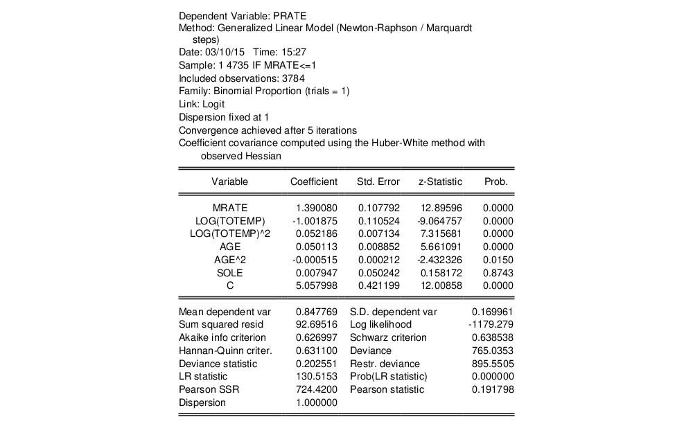
The results using the QML with GLM standard errors rely on validity of the GLM assumption for the variance given in
Equation (32.2), an assumption that may be too restrictive. We may instead estimate the equation without imposing a particular conditional variance specification by computing our estimates using a robust Huber-White sandwich method. Click on to bring up the equation dialog, select the tab, then change the from to . Click on to estimate the revised specification:
EViews reports the new method of computing the coefficient covariance in the header. The coefficient estimates are unchanged, since the alternative computation of the coefficient covariance is a post-estimation procedure, and the new standard estimates correspond the second set of standard errors in Papke and Wooldridge (Table II, column 2). Notably, the use of an alternative estimator for the coefficient covariance has little substantive effect on the results.