Count Models
Count models are employed when

takes integer values that represent the number of events that occur—examples of count data include the number of patents filed by a company, and the number of spells of unemployment experienced over a fixed time interval.
EViews provides support for the estimation of several models of count data. In addition to the standard poisson and negative binomial maximum likelihood (ML) specifications, EViews provides a number of quasi-maximum likelihood (QML) estimators for count data.
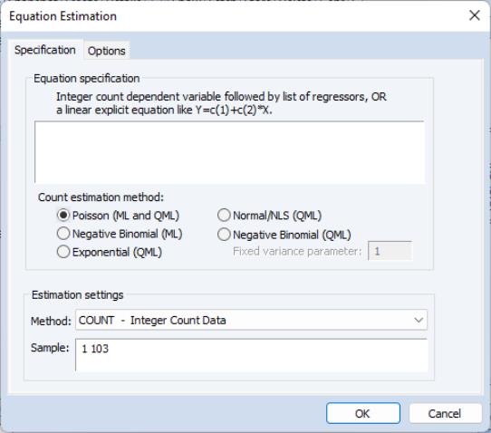
Estimating Count Models in EViews
To estimate a count data model, select from the main menu, and select as the estimation method. EViews displays the count estimation dialog into which you will enter the dependent and explanatory variable regressors, select a type of count model, and if desired, set estimation options.
There are three parts to the specification of the count model:
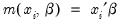
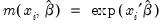
• In the upper edit field, you should list the dependent variable and the independent variables or you should provide an explicit expression for the index. The list of explanatory variables specifies a model for the conditional mean of the dependent variable:
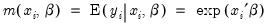 | (31.50) |
• Next, click on Options and, if desired, change the default estimation algorithm, convergence criterion, starting values, and method of computing the coefficient covariance.
• Lastly, select one of the entries listed under count estimation method, and if appropriate, specify a value for the variance parameter. Details for each method are provided in the following discussion.
Poisson Model
For the Poisson model, the conditional density of

given

is:
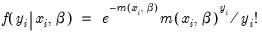 | (31.51) |
where

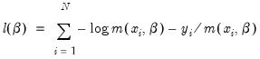
is a non-negative integer valued random variable. The maximum likelihood estimator (MLE) of the parameter

is obtained by maximizing the log likelihood function:
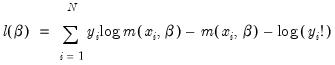 | (31.52) |
Provided the conditional mean function is correctly specified and the conditional distribution of

is Poisson, the MLE

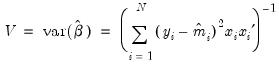
is consistent, efficient, and asymptotically normally distributed, with coefficient variance matrix consistently estimated by the inverse of the Hessian:
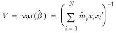 | (31.53) |
where
. Alternately, one could estimate the coefficient covariance using the inverse of the outer-product of the scores:
 | (31.54) |
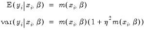
The Poisson assumption imposes restrictions that are often violated in empirical applications. The most important restriction is the equality of the (conditional) mean and variance:
 | (31.55) |
If the mean-variance equality does not hold, the model is misspecified. EViews provides a number of other estimators for count data which relax this restriction.
We note here that the Poisson estimator may also be interpreted as a quasi-maximum likelihood estimator. The implications of this result are discussed below.
Negative Binomial (ML)
One common alternative to the Poisson model is to estimate the parameters of the model using maximum likelihood of a negative binomial specification. The log likelihood for the negative binomial distribution is given by:
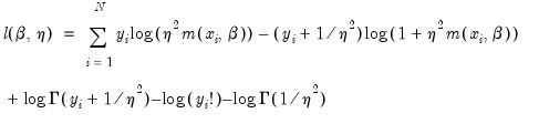 | (31.56) |
where

is a variance parameter to be jointly estimated with the conditional mean parameters

. EViews estimates the log of

, and labels this parameter as the “SHAPE” parameter in the output. Standard errors are computed using the inverse of the information matrix.
The negative binomial distribution is often used when there is
overdispersion in the data, so that
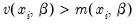
, since the following moment conditions hold:
 | (31.57) |

is therefore a measure of the extent to which the conditional variance exceeds the conditional mean.
Consistency and efficiency of the negative binomial ML requires that the conditional distribution of

be negative binomial.
Quasi-maximum Likelihood (QML)
We can perform maximum likelihood estimation under a number of alternative distributional assumptions. These quasi-maximum likelihood (QML) estimators are robust in the sense that they produce consistent estimates of the parameters of a correctly specified conditional mean, even if the distribution is incorrectly specified.
This robustness result is exactly analogous to the situation in ordinary regression, where the normal ML estimator (least squares) is consistent, even if the underlying error distribution is not normally distributed. In ordinary least squares, all that is required for consistency is a correct specification of the conditional mean
. For QML count models, all that is required for consistency is a correct specification of the conditional mean

.
The estimated standard errors computed using the inverse of the information matrix will not be consistent unless the conditional distribution of

is correctly specified. However, it is possible to estimate the standard errors in a robust fashion so that we can conduct valid inference, even if the distribution is incorrectly specified.
EViews provides options to compute two types of robust standard errors. Click
Options in the Equation Specification dialog box and mark the
Robust Covariance option. The
Huber/White option computes QML standard errors, while the
GLM option computes standard errors corrected for overdispersion. See
“Technical Notes” for details on these options.
Further details on QML estimation are provided by Gourioux, Monfort, and Trognon (1994a, 1994b). Wooldridge (1997) provides an excellent summary of the use of QML techniques in estimating parameters of count models. See also the extensive related literature on Generalized Linear Models (McCullagh and Nelder, 1989).
Poisson
The Poisson MLE is also a QMLE for data from alternative distributions. Provided that the conditional mean is correctly specified, it will yield consistent estimates of the parameters

of the mean function. By default, EViews reports the ML standard errors. If you wish to compute the QML standard errors, you should click on
Options, select
Robust Covariances, and select the desired covariance matrix estimator.
Exponential
The log likelihood for the exponential distribution is given by:
 | (31.58) |
As with the other QML estimators, the exponential QMLE is consistent even if the conditional distribution of

is not exponential, provided that

is correctly specified. By default, EViews reports the robust QML standard errors.
Normal
The log likelihood for the normal distribution is:
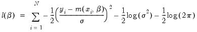 | (31.59) |
For
fixed 
and correctly specified

, maximizing the normal log likelihood function provides consistent estimates even if the distribution is not normal. Note that maximizing the normal log likelihood for a fixed

is equivalent to minimizing the sum of squares for the nonlinear regression model:
 | (31.60) |
EViews sets

by default. You may specify any other (positive) value for

by changing the number in the
Fixed variance parameter field box. By default, EViews reports the robust QML standard errors when estimating this specification.
Negative Binomial
If we maximize the negative binomial log likelihood, given above, for
fixed 
, we obtain the QMLE of the conditional mean parameters

. This QML estimator is consistent even if the conditional distribution of

is not negative binomial, provided that

is correctly specified.
EViews sets

by default, which is a special case known as the geometric distribution. You may specify any other (positive) value by changing the number in the
Fixed variance parameter field box. For the negative binomial QMLE, EViews by default reports the robust QMLE standard errors.
Views of Count Models
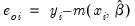
EViews provides a full complement of views of count models. You can examine the estimation output, compute frequencies for the dependent variable, view the covariance matrix, or perform coefficient tests. Additionally, you can select and pick from a number of views describing the ordinary residuals
, or you can examine the correlogram and histogram of these residuals. For the most part, all of these views are self-explanatory.
Note, however, that the LR test statistics presented in the summary statistics at the bottom of the equation output, or as computed under the have a known asymptotic distribution only if the conditional distribution is correctly specified. Under the weaker GLM assumption that the true variance is proportional to the nominal variance, we can form a quasi-likelihood ratio,
, where

is the estimated proportional variance factor. This QLR statistic has an asymptotic

distribution under the assumption that the mean is correctly specified and that the variances follow the GLM structure. EViews does not compute the QLR statistic, but it can be estimated by computing an estimate of

based upon the standardized residuals. We provide an example of the use of the QLR test statistic below.
If the GLM assumption does not hold, then there is no usable QLR test statistic with a known distribution; see Wooldridge (1997).
Procedures for Count Models
Most of the procedures are self-explanatory. Some details are required for the forecasting and residual creation procedures.
• provides you the option to forecast the dependent variable

or the predicted linear index

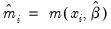
. Note that for all of these models the forecasts of

are given by
where
.
• provides the following three types of residuals for count models:
Ordinary | |
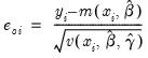
Standardized (Pearson) | |
Generalized |  =(varies) |
where the

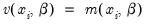
represents any additional parameters in the variance specification. Note that the specification of the variances may vary significantly between specifications. For example, the Poisson model has
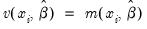
, while the exponential has
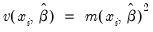
.
The generalized residuals can be used to obtain the score vector by multiplying the generalized residuals by each variable in

. These scores can be used in a variety of LM or conditional moment tests for specification testing; see Wooldridge (1997).
Demonstrations
A Specification Test for Overdispersion
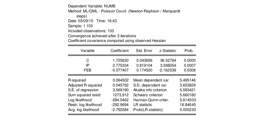
Consider the model:
 | (31.61) |
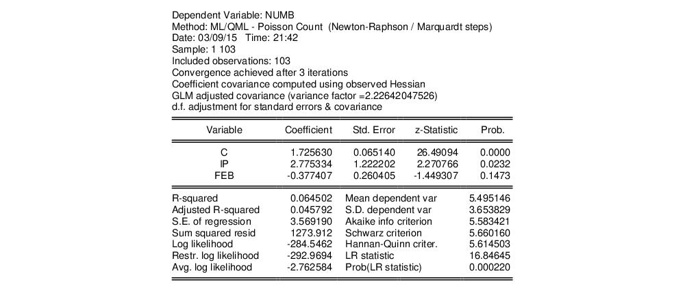
where the dependent variable NUMB is the number of strikes, IP is a measure of industrial production, and FEB is a February dummy variable, as reported in Kennan (1985, Table 1) and provided in the workfile “Strike.WF1”.
The results from Poisson estimation of this model are presented below:
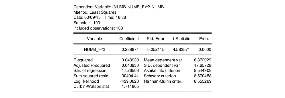
Cameron and Trivedi (1990) propose a regression based test of the Poisson restriction
. To carry out the test, first estimate the Poisson model and obtain the fitted values of the dependent variable. Click and provide a name for the forecasted dependent variable, say NUMB_F. The test is based on an auxiliary regression of

on

and testing the significance of the regression coefficient. For this example, the test regression can be estimated by the command:
equation testeq.ls (numb-numb_f)^2-numb numb_f^2
yielding the following results:
The t-statistic of the coefficient is highly significant, leading us to reject the Poisson restriction. Moreover, the estimated coefficient is significantly positive, indicating overdispersion in the residuals.
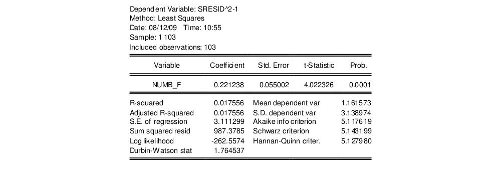
An alternative approach, suggested by Wooldridge (1997), is to regress

, on

. To perform this test, select and select
Standardized. Save the results in a series, say SRESID. Then estimating the regression specification:
sresid^2-1 numbf
yields the results:
Both tests suggest the presence of overdispersion, with the variance approximated by roughly
.
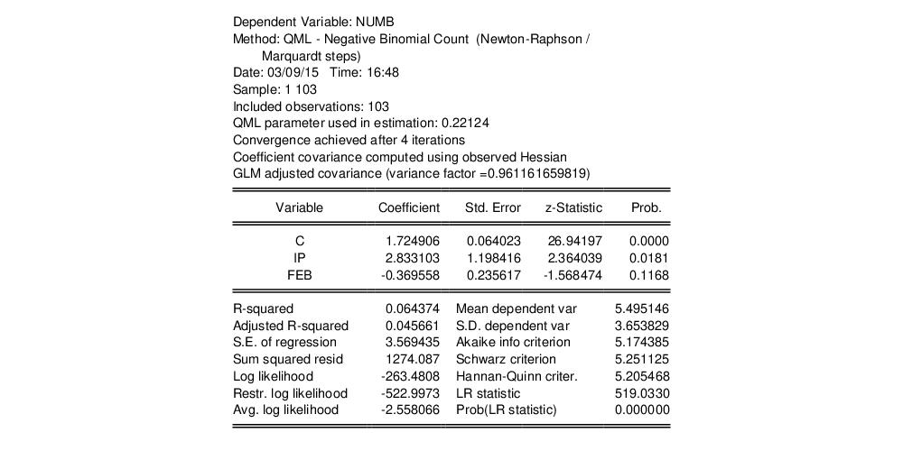
Given the evidence of overdispersion and the rejection of the Poisson restriction, we will re-estimate the model, allowing for mean-variance inequality. Our approach will be to estimate the two-step negative binomial QMLE specification (termed the
quasi-generalized pseudo-maximum likelihood estimator by Gourieroux, Monfort, and Trognon (1984a, 1984b)) using the estimate of

from the Wooldridge test derived above. To compute this estimator, simply select
Negative Binomial (QML) and enter “0.221238” in the edit field for
Fixed variance parameter.
We will use the GLM variance calculations, so you should click on Option in the dialog and choose the GLM option in the Covariance method dropdown menu. The estimation results are shown below:
The negative binomial QML should be consistent, and under the GLM assumption, the standard errors should be consistently estimated. It is worth noting that the coefficient on FEB, which was strongly statistically significant in the Poisson specification, is no longer significantly different from zero at conventional significance levels.
Quasi-likelihood Ratio Statistic
As described by Wooldridge (1997), specification testing using likelihood ratio statistics requires some care when based upon QML models. We illustrate here the differences between a standard LR test for significant coefficients and the corresponding QLR statistic.
From the results above, we know that the overall likelihood ratio statistic for the Poisson model is 16.85, with a corresponding
p-value of 0.0002. This statistic is valid under the assumption that

is specified correctly and that the mean-variance equality holds.
We can decisively reject the latter hypothesis, suggesting that we should derive the QML estimator with consistently estimated covariance matrix under the GLM variance assumption. While EViews currently does not automatically adjust the LR statistic to reflect the QML assumption, it is easy enough to compute the adjustment by hand. Following Wooldridge, we construct the QLR statistic by dividing the original LR statistic by the estimated GLM variance factor. (Alternately, you may use the GLM estimators for count models described in
“Generalized Linear Models”, which do compute the QLR statistics automatically.)
Suppose that the estimated QML equation is named EQ1 and that the results are given by:
Note that when you select the GLM robust standard errors, EViews reports the estimated, here d.f. corrected, variance factor. Then you can use EViews to compute p-value associated with this statistic, placing the results in scalars using the following commands:
scalar qlr = eq1.@lrstat/2.226420477
scalar qpval = 1-@cchisq(qlr, 2)
You can examine the results by clicking on the scalar objects in the workfile window and viewing the results. The QLR statistic is 7.5666, and the p-value is 0.023. The statistic and p-value are valid under the weaker conditions that the conditional mean is correctly specified, and that the conditional variance is proportional (but not necessarily equal) to the conditional mean.