Ordered Dependent Variable Models
EViews estimates the ordered-response model of Aitchison and Silvey (1957) under a variety of assumptions about the latent error distribution. In ordered dependent variable models, the observed

denotes outcomes representing ordered or ranked categories. For example, we may observe individuals who choose between one of four educational outcomes: less than high school, high school, college, advanced degree. Or we may observe individuals who are employed, partially retired, or fully retired.
As in the binary dependent variable model, we can model the observed response by considering a latent variable

that depends linearly on the explanatory variables

:
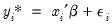 | (31.18) |
where is

are independent and identically distributed random variables. The observed

is determined from

using the rule:
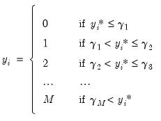 | (31.19) |
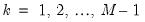
so that there are

distinct categories. It is worth noting that the actual values chosen to represent the categories in

are completely arbitrary. All the ordered specification requires is for ordering to be preserved so that

implies that

.
It follows that the probabilities of observing each value of

are given by
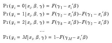 | (31.20) |
where

is the cumulative distribution function of

.
The threshold values

are estimated along with the

coefficients by maximizing the log likelihood function:
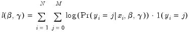 | (31.21) |
where

is an indicator function which takes the value 1 if the argument is true, and 0 if the argument is false. By default, EViews uses analytic second derivative methods to obtain parameter and variance matrix of the estimated coefficient estimates (see
“Quadratic hill-climbing (Goldfeld-Quandt)”).
Estimating Ordered Models in EViews
Suppose that the dependent variable DANGER is an index ordered from 1 (least dangerous animal) to 5 (most dangerous animal). We wish to model this ordered dependent variable as a function of the explanatory variables, BODY, BRAIN and SLEEP. Note that the values that we have assigned to the dependent variable are not relevant, only the ordering implied by those values. EViews will estimate an identical model if the dependent variable is recorded to take the values 1, 2, 3, 4, 5 or 10, 234, 3243, 54321, 123456.
(The data, which are from Allison, Truett, and D.V. Cicchetti (1976).“Sleep in Mammals: Ecological and Constitutional Correlates,” Science, 194, 732-734, are available in the “Order.WF1” dataset. A more complete version of the data may be obtained from StatLib: http://lib.stat.cmu.edu/datasets/sleep).
To estimate this model, select from the main menu. From the dialog, select estimation method ORDERED. The standard estimation dialog will change to match this specification.
There are three parts to specifying an ordered variable model: the equation specification, the error specification, and the sample specification. First, in the Equation specification field, you should type the name of the ordered dependent variable followed by the list of your regressors, or you may enter an explicit expression for the index. In our example, you will enter:
danger body brain sleep
Also keep in mind that:
• A separate constant term is not separately identified from the limit points

, so EViews will ignore any constant term in your specification. Thus, the model:
danger c body brain sleep
is equivalent to the specification above.
• EViews requires the dependent variable to be integer valued, otherwise you will see an error message, and estimation will stop. This is not, however, a serious restriction, since you can easily convert the series into an integer using @round, @floor or @ceil in an auto-series expression.
Next, select between the ordered logit, ordered probit, and the ordered extreme value models by choosing one of the three distributions for the latent error term.
Lastly, specify the estimation sample.
You may click on the tab to set the iteration limit, convergence criterion, optimization algorithm, and most importantly, method for computing coefficient covariances. See
“Technical Notes” for a discussion of these methods.
Now click on OK, EViews will estimate the parameters of the model using iterative procedures.
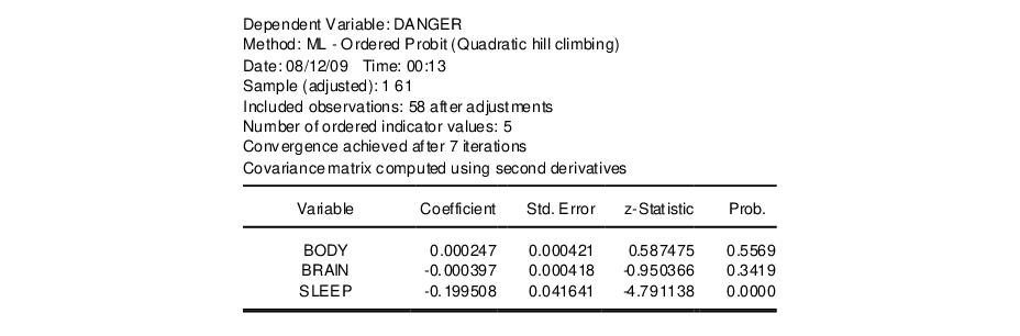
Once the estimation procedure converges, EViews will display the estimation results in the equation window. The first part of the table contains the usual header information, including the assumed error distribution, estimation sample, iteration and convergence information, number of distinct values for

, and the method of computing the coefficient covariance matrix.
Below the header information are the coefficient estimates and asymptotic standard errors, and the corresponding z-statistics and significance levels. The estimated coefficients of the ordered model must be interpreted with care (see Greene (2008, section 23.10) or Johnston and DiNardo (1997, section 13.9)).
The
sign of

shows the direction of the change in the probability of falling in the endpoint rankings (

or

) when

changes. Pr(

) changes in the
opposite direction of the sign of

and Pr(

) changes in the
same direction as the sign of

. The effects on the probability of falling in any of the middle rankings are given by:
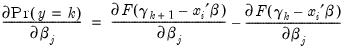 | (31.22) |
for
. It is impossible to determine the signs of these terms,
a priori.
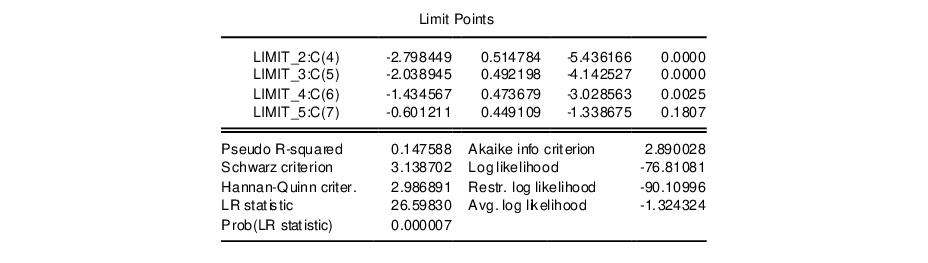
The lower part of the estimation output, labeled “Limit Points”, presents the estimates of the

coefficients and the associated standard errors and probability values:
Note that the coefficients are labeled both with the identity of the limit point, and the coefficient number. Just below the limit points are the summary statistics for the equation.
Estimation Problems
Most of the previous discussion of estimation problems for binary models (
“Estimation Problems”) also holds for ordered models. In general, these models are well-behaved and will require little intervention.
There are cases, however, where problems will arise. First, EViews currently has a limit of 750 total coefficients in an ordered dependent variable model. Thus, if you have 25 right-hand side variables, and a dependent variable with 726 distinct values, you will be unable to estimate your model using EViews.
Second, you may run into identification problems and estimation difficulties if you have some groups where there are very few observations. If necessary, you may choose to combine adjacent groups and re-estimate the model.
EViews may stop estimation with the message “Parameter estimates for limit points are non-ascending”, most likely on the first iteration. This error indicates that parameter values for the limit points were invalid, and that EViews was unable to adjust these values to make them valid. Make certain that if you are using user defined parameters, the limit points are strictly increasing. Better yet, we recommend that you employ the EViews starting values since they are based on a consistent first-stage estimation procedure, and should therefore be quite well-behaved.
Views of Ordered Equations
EViews provides you with several views of an ordered equation. As with other equations, you can examine the specification and estimated covariance matrix as well as perform Wald and likelihood ratio tests on coefficients of the model. In addition, there are several views that are specialized for the ordered model:
• Dependent Variable Frequencies — computes a one-way frequency table for the ordered dependent variable for the observations in the estimation sample. EViews presents both the frequency table and the cumulative frequency table in levels and percentages.
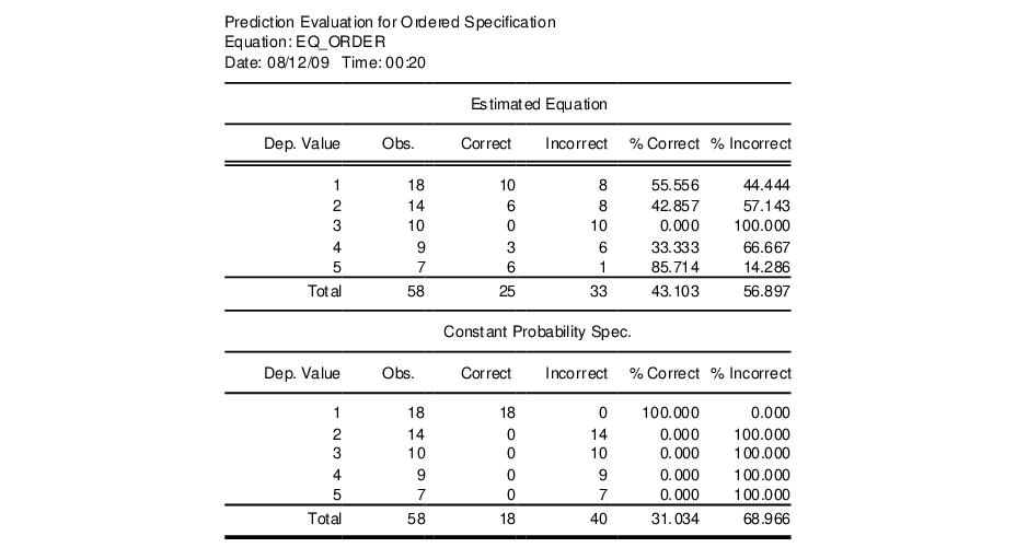
• Prediction Evaluation— classifies observations on the basis of the predicted response. EViews performs the classification on the basis of the category with the maximum predicted probability.
The first portion of the output shows results for the estimated equation and for the constant probability (no regressor) specifications.
Each row represents a distinct value for the dependent variable. The “Obs” column indicates the number of observations with that value. Of those, the number of “Correct” observations are those for which the predicted probability of the response is the highest. Thus, 10 of the 18 individuals with a DANGER value of 1 were correctly specified. Overall, 43% of the observations were correctly specified for the fitted model versus 31% for the constant probability model.
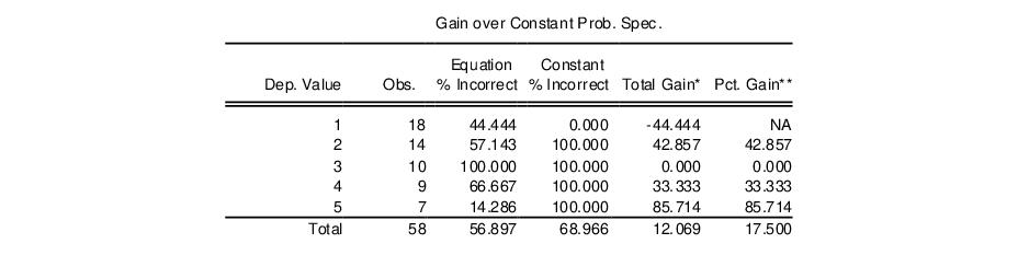
The bottom portion of the output shows additional statistics measuring this improvement
Note the improvement in the prediction for DANGER values 2, 4, and especially 5 comes from refinement of the constant only prediction of DANGER=1.
Procedures for Ordered Equations
Make Ordered Limit Vector/Matrix
The full set of coefficients and the covariance matrix may be obtained from the estimated equation in the usual fashion (see
“Working With Equation Statistics”). In some circumstances, however, you may wish to perform inference using only the estimates of the

coefficients and the associated covariances.
The and procedures provide a shortcut method of obtaining the estimates associated with the

coefficients. The first procedure creates a vector (using the next unused name of the form LIMITS01, LIMITS02, etc.) containing the estimated

coefficients. The latter procedure creates a symmetric matrix containing the estimated covariance matrix of the

. The matrix will be given an unused name of the form VLIMITS01, VLIMITS02, etc., where the “V” is used to indicate that these are the variances of the estimated limit points.
Forecasting using Models
You cannot forecast directly from an estimated ordered model since the dependent variable represents categorical or rank data. EViews does, however, allow you to forecast the probability associated with each category. To forecast these probabilities, you must first create a model. Choose and EViews will open an untitled model window containing a system of equations, with a separate equation for the probability of each ordered response value.
To forecast from this model, simply click the Solve button in the model window toolbar. If you select Scenario 1 as your solution scenario, the default settings will save your results in a set of named series with “_1” appended to the end of the each underlying name. See
“Models” for additional detail on modifying and solving models.
For this example, the series
I_DANGER_1 will contain the fitted linear index

. The fitted probability of falling in category 1 will be stored as a series named
DANGER_1_1, the fitted probability of falling in category 2 will be stored as a series named
DANGER_2_1, and so on. Note that for each observation, the fitted probability of falling in each of the categories sums up to one.
Make Residual Series
The generalized residuals of the ordered model are the derivatives of the log likelihood with respect to a hypothetical unit-

variable. These residuals are defined to be uncorrelated with the explanatory variables of the model (see Chesher and Irish (1987), and Gourieroux, Monfort, Renault and Trognon (1987) for details), and thus may be used in a variety of specification tests.
To create a series containing the generalized residuals, select , enter a name or accept the default name, and click . The generalized residuals for an ordered model are given by:
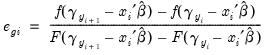 | (31.23) |
where

, and

.