| | |
Beta | @cbeta(x,a,b[,n]), @dbeta(x,a,b), @qbeta(p,a,b), @rbeta(a,b) | for  and for  , where  is the @beta function. |
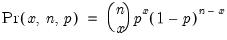
Binomial | @cbinom(x,n,p), @dbinom(x,n,p), @qbinom(s,n,p), @rbinom(n,p) | if  , and 0 otherwise, for  . |
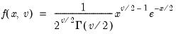
Chi-square | @cchisq(x,v[,n]), @dchisq(x,v), @qchisq(p,v), @rchisq(v) | where  , and  . Note that the degrees of freedom parameter  need not be an integer. In addition, the @chisq(x,v) function may be used to obtain the p-values directly. |
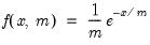
Exponential | @cexp(x,m[,n]), @dexp(x,m), @qexp(p,m), @rexp(m) | for  , and  . |
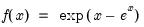
Extreme Value (Type I-minimum) | @cextreme(x[,n]), @dextreme(x), @qextreme(p), @cloglog(p), @rextreme | for  . |
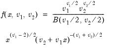
F-distribution | @cfdist(x,v1,v2[,n]), @dfdist(x,v1,v2), @qfdist(p,v1,v2), @rfdist(v1,v1) | where  , and  . Note that the functions allow for fractional degrees of freedom parameters  and  . |
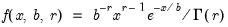
Gamma | @cgamma(x,b,r[,n]), @dgamma(x,b,r), @qgamma(p,b,r), @rgamma(b,r) | where  , and  . |
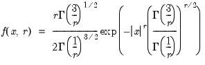
Generalized Error | @cged(x,r[,n]), @dged(x,r), @qged(p,r), @rged(r) | where  , and  . |
Laplace | @claplace(x[,n]), @dlaplace(x), @qlaplace(x), @rlaplace | for  . |
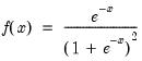
Logistic | @clogistic(x[,n]), @dlogistic(x), @qlogistic(p), @rlogistic | for  . |
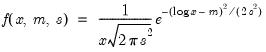
Log-normal | @clognorm(x,m,s[,n]), @dlognorm(x,m,s), @qlognorm(p,m,s), @rlognorm(m,s) | |
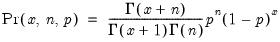
Negative Binomial | @cnegbin(x,n,p), @dnegbin(x,n,p), @qnegbin(s,n,p), @rnegbin(n,p) | if 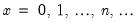 , and 0 otherwise, for  . |
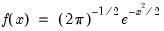
Normal (Gaussian) | @cnorm(x[,n]), @dnorm(x), @qnorm(p), @rnorm, nrnd, @logcnorm | for  . @logcnorm is a more numerically stable function for the computation of @log(@cnorm(x)) |
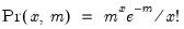
Poisson | @cpoisson(x,m), @dpoisson(x,m), @qpoisson(p,m), @rpoisson(m) | if  , and 0 otherwise, for  . |
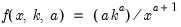
Pareto | @cpareto(x,k,a[,n]), @dpareto(x,k,a), @qpareto(p,k,a), @rpareto(k,a) | for location parameter  and shape parameter  . |
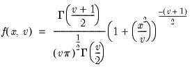
Student's  ‑distribution | @ctdist(x,v[,n]), @dtdist(x,v), @qtdist(p,v), @rtdist(v) | for  , and  . Note that  , yields the Cauchy distribution. |
Uniform | @cunif(x,a,b), @dunif(x,a,b), @qunif(p,a,b), @runif(a,b), rnd | for  and  . |
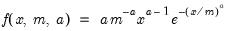
Weibull | @cweib(x,m,a[,n]), @dweib(x,m,a), @qweib(p,m,a), @rweib(m,a) | where  , and  . |
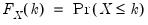 . The quantile functions will return the smallest value where the CDF evaluated at the value equals or exceeds the probability of interest:
  , where
  . The inequalities are only relevant for discrete distributions.
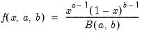

 ,
,  , and
, and  .
.

 and
and  for a distribution with means 0, variances 1, and correlation
  .
. . This form is more efficient when performing multiple draws from the same distribution (compute the Cholesky once, but sample many times).
 . This form is more efficient than explicitly inverting
  to supply
  .
. . This form combines the efficiencies of the above forms.
 with
with 
 , where
 is positive semi-definite.
 , where
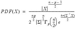 ,
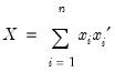
, are
are  positive definite matrices, and the degrees-of-freedom parameter
  and
and  .
. , i.e.,
  ,
, ,
,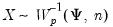 , where
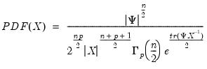 ,
, are
are  positive definite matrices, and the degrees-of-freedom parameter
  and
and  .
. , so there are many relations among the Wishart and inverse Wishart functions, e.g.,
  degrees of freedom exceeds
  :
: numerator degrees of freedom and
  denominator degrees of freedom exceeds
  :
:  degrees of freedom exceeds
  in absolute value (two-sided