An Example
As an example of using MIDAS regression in EViews, we analyze data used by Armesto, Engemann, and Owyang (2010). The data consists of log-differenced, seasonally adjusted quarterly real GDP between 1947 and 2011 and log-differenced monthly total non-farm payroll employment from 1939 to 2011. These data are in the workfile “Midas.WF1” with the real GDP data in series REALGDP on page “QuarterlyPage”, and the employment data in series EMP on page “MonthlyPage”.
Beta Weighting
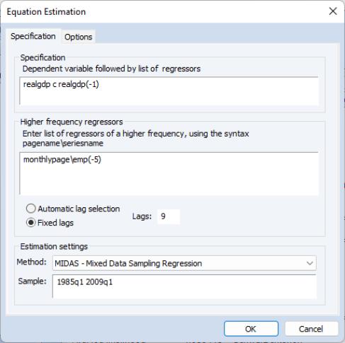
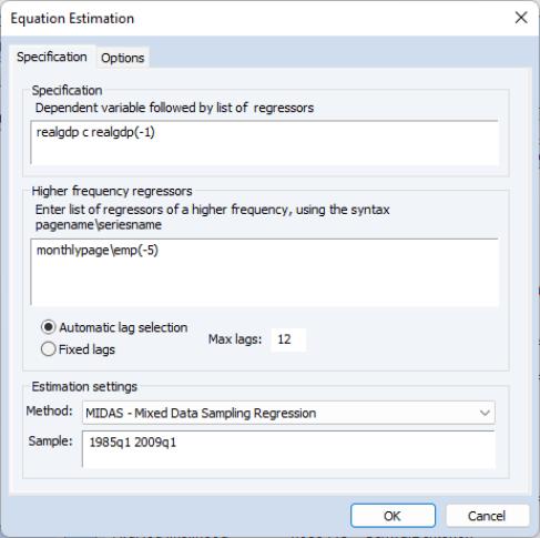
We estimate a MIDAS model with real GDP as the dependent variable and a lagged value of real GDP as a regressor. Only data between 1985 and 2009q1 are used. Monthly employment with 9 lags is used as a set of higher-frequency regressors. The employment data lags are off-set by 5 months (i.e., to explain Quarter 1 real GDP, employment data from the previous year’s February through October are used).
We use the beta weighting method, while restricting the endpoints coefficient

to be zero. The following dialog settings reflect this equation specification:
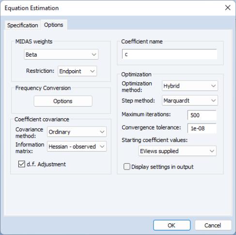
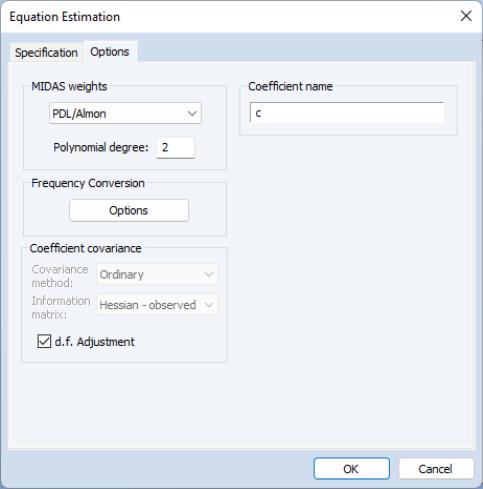
and the associated options
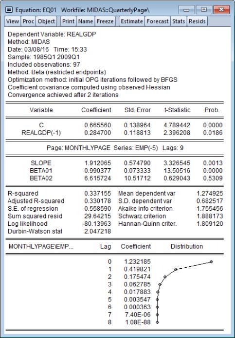
The results of this estimation are given by
The top portion of the output describes the estimation sample, MIDAS method, and other estimation settings. Here we see that beta weighting with restricted endpoints (

). Estimation uses the hybrid method of initial OPG iterations followed by BFGS estimation, with the coefficient covariance computed using the inverse of the negative Hessian.
The first section displays coefficients, standard errors, and t-statistics for the low frequency regressors. These results show standard regression output.
Next, we display the results for the high frequency variables. First, we describe the page and name of the variable and the number lags

used in the low frequency regression. Here, we are using EMP(-5) from the “monthlypage” and allowing for 9 high frequency lags of this variable in the low frequency regression.
The coefficient results for the common SLOPE coefficient (

) and the free MIDAS beta weight coefficients (

) are displayed directly below.
First, we see that monthly EMP(-5) has an overall positive effect on REALGDP as the SLOPE coefficient is a statistically significant 1.91.
The actual lag coefficients are obtained by applying weights to this overall slope. The shape of the weight function is determined by the remaining MIDAS coefficients. The

coefficient, labeled BETA01, is very close to 1, so that the lag pattern depends primarily on BETA02 (

).
The large positive estimate of

, is statistically different from 1, and value of 6.62, implies that the lag pattern is sharply decreasing as shown in the lag coefficient graph at the bottom of the output. We conclude that the coefficient that the zero high frequency lag of employment has a large impact on real GDP, but the effect dies off pretty quickly.
The endpoint coefficient

has been restricted to be zero so that it does not appear in the output.
The remaining output consists of the standard summary statistics and diagnostics.
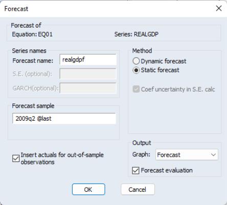
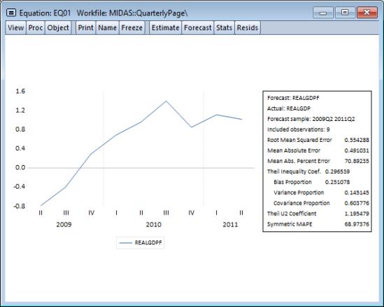
To continue our example, we wish to perform a static forecast over the period after the estimation sample (2009q2) to the end of the workfile (2011q2). To forecast from our MIDAS equation, we do so in the usual manner, by first clicking the button:
and filling out the resulting dialog with the appropriate settings. Clicking on performs the forecast:
Almon Weighting
As a second example we will estimate the same model, but this time using the Almon weighting method, with a second degree polynomial, and we instruct EViews to select the most appropriate number of lags for employment (up to a maximum of 12):
and
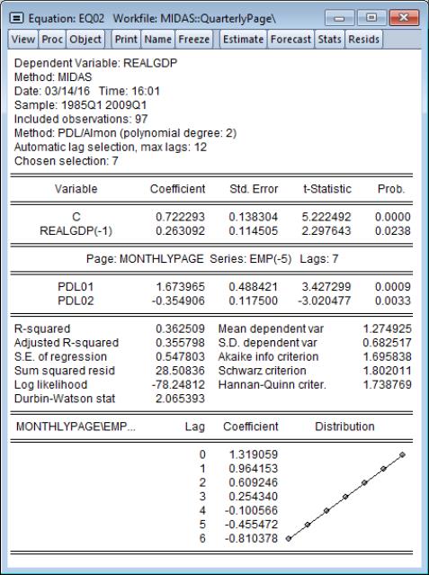
Clicking on estimates the specified equation, and displays the results:
As with the beta weighting model estimated above, the overall effect of high frequency EMP(-5) on REALGDP is positive and decreasing in the lags. However, in contrast with the beta weights estimates, the Almon weights lag coefficients do not decline sharply; in fact, the pattern appears to be roughly linear.
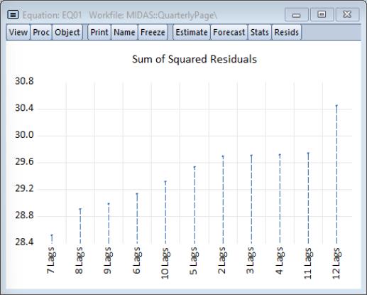
Note that the MIDAS variable description line shows that EViews chose 7 as the most appropriate high frequency lag length. Clicking on displays a graph of the sum of squared residuals from each of the different lag selections:
providing clear evidence that 7 is the optimal lag.