MIDAS Estimation in EViews
With built-in tools for working with multi-frequency data and an intrinsic understanding of the relationship between various time series frequencies, EViews offers an ideal platform for MIDAS estimation.
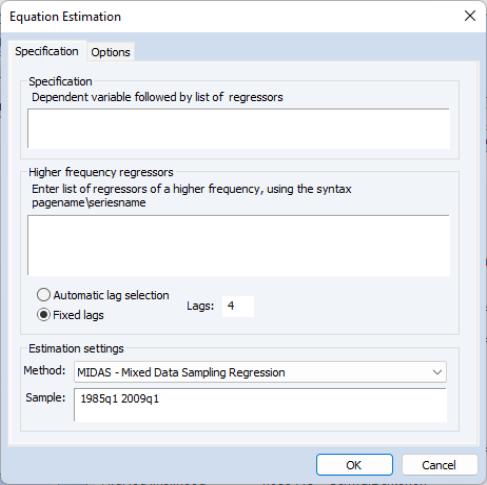
To perform MIDAS estimation in EViews, open the equation dialog by selecting , or by selecting and then selecting from the dropdown menu to bring up the MIDAS estimation dialog:
Specification
The tab is used to specify the variables of and form of the MIDAS equation and to set the estimation sample.
The edit field is used to specify the low frequency dependent variable followed by a list of low frequency regressors from the same page as the dependent variable. The low frequency regressors should include any desired lags of the dependent variable. Note that explicit ARMA terms are not permitted in this estimation method.
The edit field is used to specify the higher-frequency regressors. The syntax for these variable is pagename\seriesname where pagename is the name of the page containing the series, and seriesname is the name of the series. Note also that series expressions are allowed, e.g. “mypage\log(x)”.
You may specify more than one higher-frequency series, and those series may be of different frequencies from different pages. However, we caution you that using more than one high frequency regressor oftens leads to multicollinearity issues and, in the case of the non-linear weighting, increases the complexity of estimation dramatically. An alternative approach suggested by Andreou, et al. (2013) would be to estimate several univariate models and then use forecast combination to produce a final forecast.
Date Timing
When specifying your high frequency variable, care should must be taken to ensure that you refer to the correct observations from the higher frequency page.
To illustrate, let’s assume our dependent variable, Y, is quarterly, and our regressor, X, is monthly. We would like to use 4 lags (months) of X to explain each quarter of Y. EViews will use the 4 months up to, and including, the last month of the corresponding quarter. Quarter 1 will thus be explained by March, February, January and December. Quarter 2 will be explained by June, May, April and March.
If you wish to use different sets of months, you can use the lag operator when specifying the regressor. In our example, if we want Quarter 1 to be explained by January, December, November and October, and Quarter 2 to be explained by April, March, February and January, we would specify the regressor as “monthlypage\x(-2)”; i.e., using the second lagged values of X.
Lag Selection
All of the MIDAS estimation methods require a value for

, the number of high frequency lags to be included in the low frequency regression equation.
Just below the edit field are radio buttons that control the number of lags. You may provide a fixed number of lags by selecting the appropriate radio button and entering a value, or you can elect to determine the number of lags using minimal sum-of-squared residuals as the selection criterion. If you select the latter radio button, you will prompted to enter a value for the maximum number of lags. Note that automatic selection is only available for the Almon and Step weighting methods.
If you have entered more than one high frequency regressor you may enter a single lag or maximum lag value or you may enter a space delimited list of lags. If you enter a single value, it will be applied to all of the regressors.
As you make your choice, keep in mind that the maximum number of lags and selected lags from automatic selection will apply to all of the high frequency series.
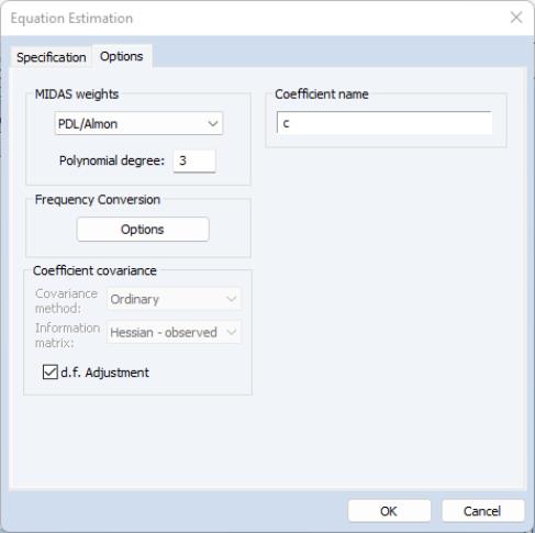
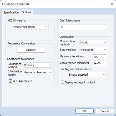
Estimation Options
The tab of the dialog lets you specify some the MIDAS weighting function along with other estimation options:
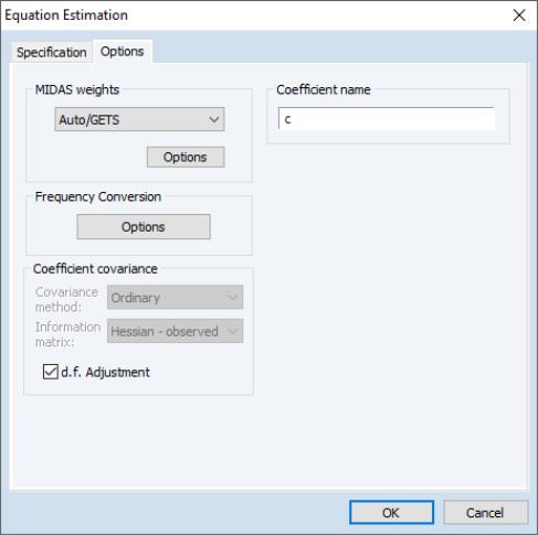
The dropdown menu controls specification of the MIDAS weighting. By default the weighting method is selected, but , , or may also be chosen:
• If you select the method, you must specify

, the degree of the Almon polynomial.
• If you select , you must specify the stepsize

.
• If you select , you may, if desired, impose restrictions on the shape parameter

, the endpoint parameter

, or both

and

. You may also specify covariance and optimization settings (
“Coefficient Covariance and Optimization”).
• If you select , and click on the button you will be prompted to specify options for the Auto/GETS selection algorithm, as well as settings for indicator saturation inclusion. See
“Variable Selection and Indicator Saturation” for extended discussion.
Frequency Conversion
The button produces a secondary dialog that allows you to change the way the different frequencies of the variables are matched. By default, EViews uses the last observation in the higher frequency periods as the 0th lag in the regression. You can change this to instruct EViews to use the first observation, or to use arbitrary date series from each page to perform the date matching.
Coefficient Covariance and Optimization
Since the and weighting methods involve non-linear estimation, selecting either of these methods will enable the andmethod options:
The e section offers standard EViews covariance settings for nonlinear regression (
“Coefficient Covariance”).
The dropdown menu offers standard EViews optimization settings for nonlinear regression (
“Optimization”), with the exception of the default . This method is a combination of the and methods, where OPG is used for an initial 50 iterations, then BFGS is used until convergence. We have found that the hybrid method often reaches convergence more successfully than OPG or BFGS alone.
For the nonlinear models, you may elect to have EViews obtain starting values, or you may specify your own.
For the exponential Almon method, EViews sets

and

, then runs OLS with those values to obtain the remaining starting values. For beta weighting, EViews sets

,

, and

, then runs OLS to obtain the remaining values. Then, if not performing shape restricted estimation, EViews updates the starting values by estimating a shape restricted beta weight model.
Variable Selection and Indicator Saturation
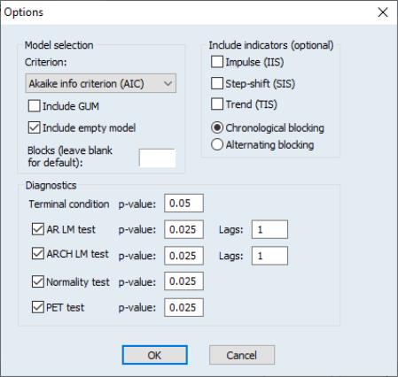
If you select in the dropdown, EViews will display an Auto/GETS button.
Clicking on this button displays a dialog showing options for variable selection and indicator saturation:
There are three sections in this dialog:
• In the section the dropdown specifies the information criteria used to select the final model from the candidate models.
The and check boxes specify whether to include the full model (including all search regressors) or the empty model (including zero search regressors) as possible candidates.
The edit field allows you to specify the number of blocks into which the search regressors will be split. Typically, if the number of search regressors is less than the number of observations in estimation, only a single block is required. However, if the number of search regressors exceeds the number of observations, they will be split into blocks. EViews will automatically determine the optimal number of blocks, but you may enter your own choice in this field to override the EViews default.
The and radio buttons determine whether the search regressors are split into blocks in chronological order (the first group of lags/indicators in the first block, followed by the next group in the second block and so on), or alternating (the first variable in the first block, second variable in the second block and so on).
• The area allows you to specify whether you would like to perform indicator detection, and the type of indicator you would like to detect.
• The options allows selection of which diagnostic tests to include, along with their p-values, and for the AR LM test and ARCH LM test, the number of lags to include.