Before describing EViews tools for working with an equation estimated using breakpoint least squares, it is important to point out that the resulting estimated equation is simply a linear regression model in which some of the variables are interacted with regime dummy variables, as in Equation (34.2). Thus, most of the discussion related to the linear regression model in “Basic Regression Analysis” and “Specification and Diagnostic Tests” applies. We focus our attention in this section on the unique aspects of the breakpoint equation.

To illustrate the output from estimation of a breakpoint equation, we employ data from Hansen’s (2001) labor productivity example. Hansen’s example uses monthly (February 1947 to April 2001) U. S. labor productivity in the manufacturing durables sector as measured by the growth rate of the ratio of the Industrial Production Index to average weekly labor hours. The data are in the series DDUR in the workfile “hansen_jep.wf1”.

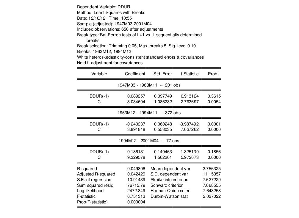
We estimate a breakpoint model with DDUR regressed on its lag DDUR(-1) and a constant. The output is presented below:

The top portion of the output shows equation specification information. As we see, the two estimated breakdates 1963m12 and 1994m12 were determined using the Bai-Perron sequential breakpoint methodology, with a maximum of 5 breaks, 5% trimming, and a test size of 0.10. Coefficient covariances for the tests and estimates are computed using White’s method with no d.f. correction.

The middle section labels each regime and shows the corresponding coefficient estimates, standard errors, and p-values.

As noted above, estimated equation is simply a linear regression model in which some of the variables are interacted with regime dummy variables. Thus, most of the equation views and procs are defined exactly as in the standard least square regression. There are, however, some specific breakpoint regression features that deserve discussion.

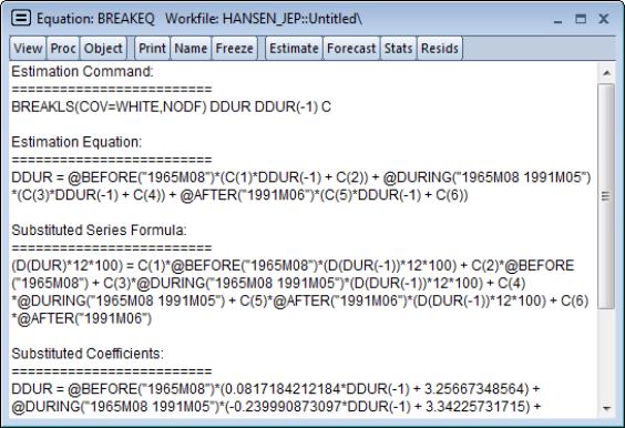
The representations view shows you the equation specification estimated by EViews:

Note in particular the use of the @before, @during, and @after functions to create regime dummy variables that interact with the regressors. You could have used these functions to specify an equivalent model using the ordinary least squares estimator.

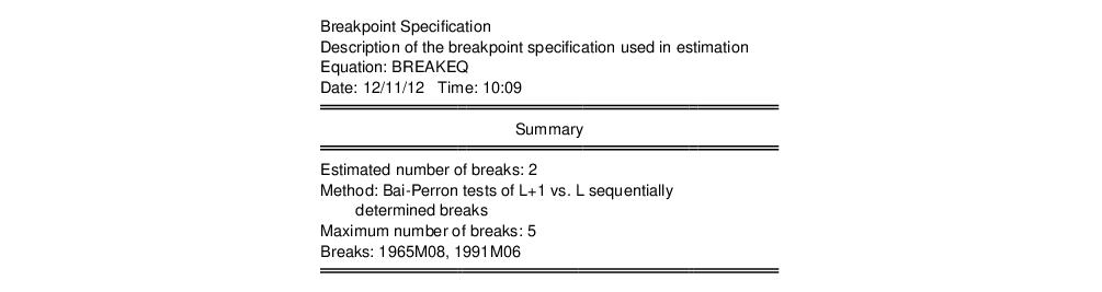
The breakpoint specification view (View/Breakpoint Specification) displays a summary of the breakpoint specification, the method used to determine the break dates, and if appropriate, re-computes and displays the test statistics used to obtain the optimal breaks.

The top portion of the output shows the breakpoint summary:

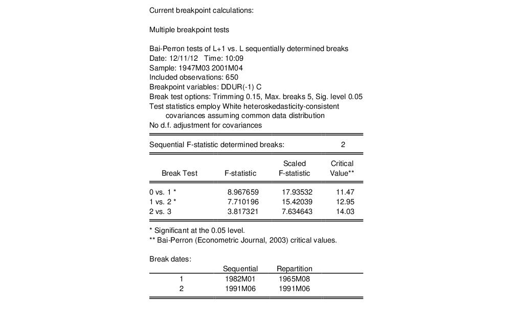
The remaining portion shows the intermediate results for the breakpoint determination:

EViews uses various methods for labeling the coefficient results in view output.

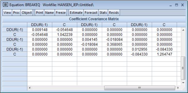
For example, the matrix-based coefficient covariance view (View/Covariance matrix) uses minimum labeling information to identify columns and rows of the covariance matrix. The coefficients are listed in the order that they appear in the equation results view, but without overt regime identification:

Here, the first to columns correspond to the coefficients on DDUR(-1) and the intercept in the first regime, the next two columns are the results for the second regime, and so on. Any non-regime specific coefficients appear at the end of the blocks of varying coefficients.

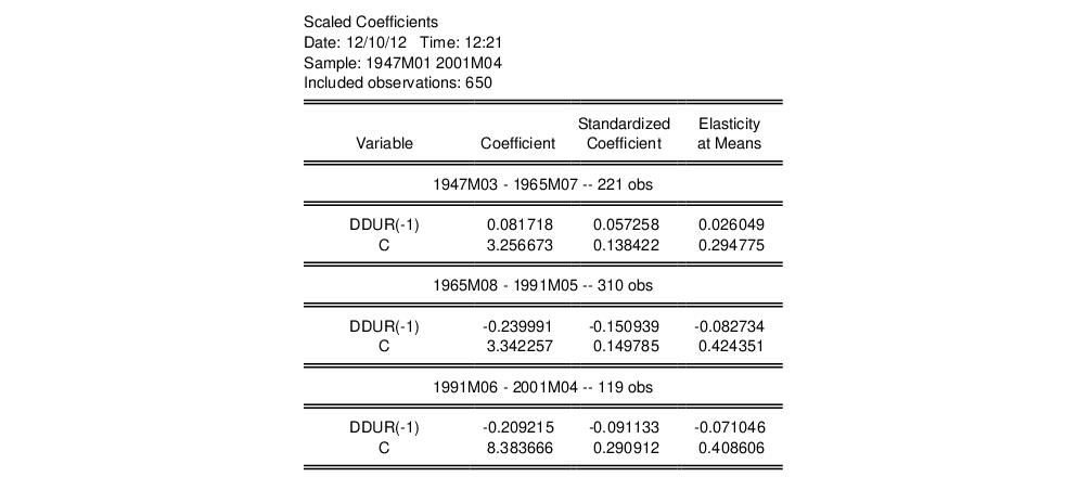
In most table output, EViews groups and labels the variables by regimes. For example, the scaled coefficients view (View/Coefficient Diagnostics/Scaled Coefficients) mirrors the format of the equation results output:

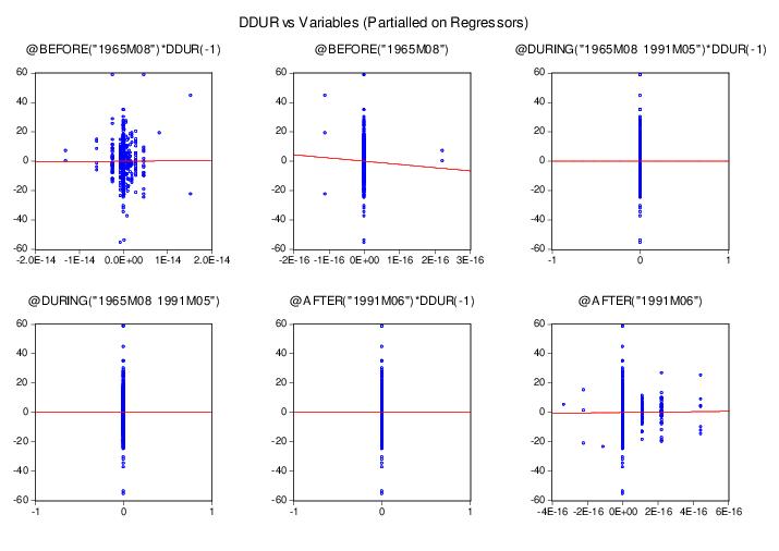
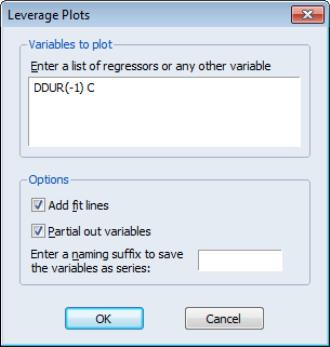
Alternately, in leverage plots (View/Stability Diagnostics/Leverage Plots...) EViews displays graphs that are labeled with the full dummy variable interaction variables previously seen in the representations view:

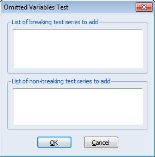
EViews dialogs will prompt you, where relevant, to indicate whether variables should have regime-specific or common coefficients. For example, the omitted variables test (View/Coefficient Diagnostics/Omitted Variables Test - Likelihood Ratio...) dialog offers separate edit fields corresponding to the two types of variables:

Similarly, if you select View/Stability Diagnostics/Leverage Plots..., EViews will prompt you to identify the variables for which you wish to display diagnostics.

Notice that in both cases, you should specify these variables in terms of the original, non-breaking variables.

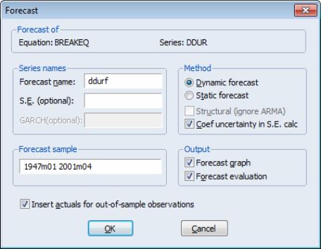
Forecasting in breakpoint least squares works the same way as in the least squares estimator. Click on the Forecast button on the toolbar or select Proc/Forecast... to bring up the dialog.

All of the settings are as in the standard linear regression case. However, it is worth noting that the saved forecast S.E. assumes a common variance across regimes even if you have relaxed this assumption in the computation of the coefficient covariances. Note also that out-of-sample forecasts will use the first regime specific coefficients for periods prior to the estimation period, and the last regime specific coefficients for periods after the estimation period.