Estimating Switching Regressions in EViews
To display the switching regression dialog, first open an equation by selecting from the main menu and select in the dropdown, or enter the command switchreg in the command line:
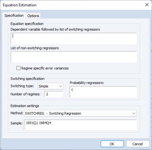
There are two tabs in this dialog. The first tab is used for basic specification of your switching regression. The second tab contains options for modifying selected features of the specification and for controlling computational aspects of the estimation.
Specification
The page contains three sections: , , and . We focus on the first two sections since the last should already be familiar.
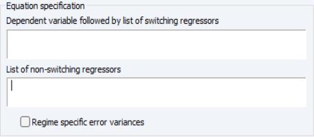
Equation Specification
The top portion of the page contains the section where you should specify the behavior of the model in the different regimes.
• You should enter the name of the dependent variable series (

) followed by any regressors with switching coefficients (

) in the first edit field.
• Regressors which have non-varying coefficients (

) should be listed in the second edit field.
• You should select the option if you wish to allow for heteroskedasticity across regimes.
You may specify dynamics by including lags of the dependent variable series as regressors or by including
AR terms to allow for serially correlated errors. Bear in mind that the dimension of the state probability vector,

, increases rapidly in

, where

is the highest AR order in the model.
Note that the dependent variable may not be specified by expression, and that the regressor lists may not contain expressions containing the dependent variable or its lags.
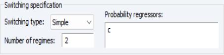
Switching Specification
The section controls the specification of the regime probabilities.
• The type dropdown allows you to choose between and switching. The default setting is to estimate a simple switching model.
• You should specify the number of regimes

in the edit field. By default, EViews assumes that you have two regimes. Bear in mind that switching models with more than a few regimes may be difficult to estimate.
• You may specify additional regressors that determine the unconditional regime probabilities (for simple switching) or the regime transition probability matrix (for Markov switching). By default, EViews sets the list so that there is a single constant term resulting in time-invariant probabilities.
Important note: the data for the probability regressors that determine the transition or regime probabilities for period  , should be located in period
  of the workfile. That is, the
  data should be in period
  of the workfile, not period
  . You may, of course, employ standard EViews lag expressions to refer to data in the previous period.
 Additional options for setting the initial regime probabilities and restricting the elements of the probability vector or transition matrix are located on the tab and described in
“Switching”.
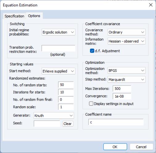
Options
Clicking on the tab displays options for modifying features of the switching specification and for controlling various aspects of the computation.
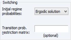
Switching
The options section may be used to specify the initial state probabilities and any restrictions to the regime probability vector or transition matrix.
Recall that evaluation of the likelihood in Markov switching and SSAR models requires presample values for the filtered probabilities (
“Initial Probabilities”). The dropdown lets you choose the method of initializing these values ( (default), , , ). If you select , you will be prompted for the name of an

-element vector in the workfile that contains the initial probabilities.
The edit field allows you to specify restrictions on the regime probabilities. Markov switching models, in particular, will sometime require restrictions on transition matrix probabilities. For example, we may have

if it is impossible to transition directly from state

to state

. Similarly, if state

is an absorbing state, then

and

for

.
To specify restrictions, you should enter the name of an

-element vector in the workfile (for a SSAR model), or an

matrix in the workfile (for Markov switching) in the edit field. The vector or matrix should contain valid probability values for elements that are restricted and NAs for elements that are to be estimated. For example, in a three regime Markov switching model where state 3 is an absorbing state, you would have
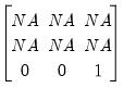 | (39.24) |
You should take care not to specify invalid or inconsistent restrictions. For example, rows of a Markov transition matrix may not be specified so that there is a single unrestricted cell since the adding up condition for the row places a restriction on that cell. Similarly, fixed values should be valid probabilities that do not have generate row sums greater than 1. EViews will detect these types of errors and will refuse to estimate the model.
In
“Regime Heteroskedasticity”, we offer an example that employs restrictions and discuss several practical issues associated with estimating the model.
Coefficient Covariance Options
EViews estimates the parameters of the likelihood using the Broyden, Fletcher, Goldfarb and Shanno (BFGS) method. By default, the coefficient covariance is computed using the d.f. corrected inverse of the negative of the observed Hessian.
You may use the dropdown to instruct EViews to use the Hessian, the outer product of the gradient (OPG) method, or a Huber-White robust covariance that forms a sandwich using the Hessian and gradients.
The checkbox may be used to remove the d.f. correction.
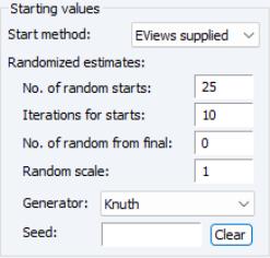
Starting Value and Iteration Options
The section contains the standard fields for setting the maximum number of iterations and convergence tolerance. By default, EViews will use the estimation settings from your global options.You may select the checkbox to display starting values and other estimation settings in the top section of your estimation output.
You may use the section to control the setting of initial parameter estimates. Switching regression models often have local roots and may be difficult to estimate so EViews offers a range of tools for choosing starting values.
Start Method
The dropdown allows you to specify a basic method for choosing starting values (, , , , , ).
The EViews supplied methods employ simple least squares coefficient estimates or the specified fraction of those estimates. AR coefficients are arbitrarily initialized to zero.
The and methods are self-explanatory, with the latter taken from the default coefficient vector specified in the dialog (typically the coefficient vector C).
Randomized Estimates
The first two edit fields under allow you to choose random starting values based on the those specified in the dropdown.
• EViews will randomly choose the number of random starts as specified in and for each random start perform the number of iterations as specified in . The coefficients with the highest likelihood value will be chosen as the starting values.
For non user-supplied starting values, EViews will, by default, generate 25 sets of random starting values and refine each with 10 iterations before choosing the best set as the starting values. By default, there is no randomization of user-supplied values.
In addition to randomizing based on the initial values, you may randomize based on the final coefficient estimates. The edit field determines the number of random coefficients to try following estimation.
• The random starting values are chosen by taking the best estimated values to date and adding random normals with scale given by the fraction of the final coefficient standard deviations. The estimates with the highest likelihood become the final estimates.
By default, EViews does not perform randomization based on the final coefficient estimates.
For both initial and final randomization, the random starting values are chosen by taking the base values and adding random normals with scale given by the fraction of the root of the estimated coefficient variances (or the scale fraction itself if the variances are not available). The random values will be generated using the specified in the dropdown and the random specified in the edit field. If a random seed is not specified, EViews will obtain one from a single draw from the generator.
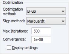
Optimization Options
You can use the dropdown menu to select a different method.
By default, EViews uses BFGS with Marquardt steps to obtain parameter estimates. You may use the dropdown to choose between , , or . The dropdown offers the choice of , , and .
The remainder of the section allows you to specify a convergence criterion and the maximum number of iterations, and to instruct EViews to display starting value and other optimization information in the output.