Estimating ARIMA and ARFIMA Models in EViews
EViews estimates ARIMA models for linear and nonlinear equations specifications defined by list or expression, and ARFIMA models for linear specifications defined by list.
Before you use the tools described in this section, you may first wish to examine your model for other signs of misspecification. Serial correlation in the errors may be evidence of serious problems with your specification. In particular, you should be on guard for an excessively restrictive specification that you arrived at by experimenting with ordinary least squares. Sometimes, adding improperly excluded variables to your regression will eliminate the serial correlation. For a discussion of the efficiency gains from the serial correlation correction and some Monte-Carlo evidence, see Rao and Griliches (l969).
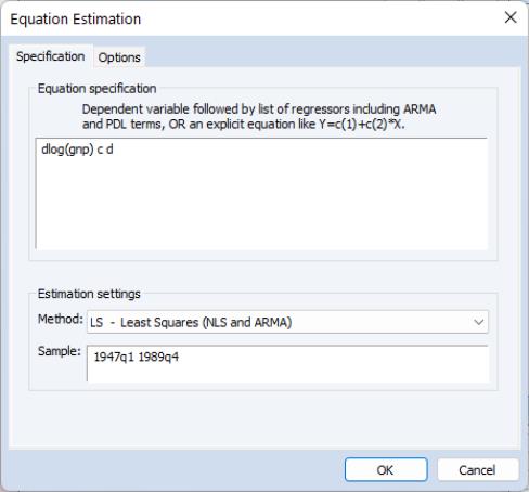
To estimate an ARMA, ARIMA, or ARFIMA model in EViews, open an equation object by clicking on or in the main EViews menu, or type equation in the command line:
Putting aside the for a moment, consider the section at the bottom of the dialog
• When estimating ARMA models, you may choose , , or in the estimation dropdown menu.
Note that some estimation techniques and methods (notable maximum likelihood and fractional integration) are only available under the least squares option.
• Enter the sample specification in the edit dialog.
As the focus of our discussion will be on the equation specification for standard ARIMA and ARFIMA models and on the corresponding settings on the tab, the remainder of our discussion will assume you have selected the method in the dropdown menu. We will make brief comments about other specifications when appropriate.
Equation Specification
EViews estimates general ARIMA and ARFIMA specifications that allow for right-hand side explanatory variables (ARIMAX and ARFIMAX).
You should enter your equation specification in the top edit field. As with other equation specifications, you may enter your equation by listing the dependent variable followed by explanatory variables and special keywords, or you may provide an explicit expression for the equation.
To specify your ARIMA model, you will:
• Difference your dependent variable, if necessary, to account for the integer order of integration.
• Describe your structural regression model (dependent variables and mean regressors) and add AR, SAR, MA, SMA terms, as necessary.
To specify your ARFIMA model you will:
• Difference your dependent variable, if necessary, to account for an integer order of integration.
• Describe your structural regression model (dependent variables and regressors) and add any ordinary and seasonal ARMA terms, if desired.
• Add the
d keyword to the specification to indicate that you would like to estimate and use a fractional difference parameter

.
Specifying AR Terms
To specify an AR term in EViews, you will use the keyword ar, followed by the desired lag or lag range enclosed in parentheses. You must explicitly instruct EViews to use each AR lag you wish to include.
First-Order AR
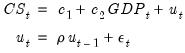
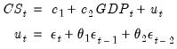
For specifications defined by list, simply add the ar keywords to the list. For example, to estimate a simple consumption function with AR(1) errors, and enter your list of variables as usual, adding the keyword expression AR(1) to the end of your list.
For the specification:
 | (24.39) |
with the series CS and GDP in the workfile, you may specify your equation as:
cs c gdp ar(1)
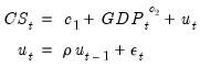
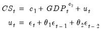
For specifications defined by expression, specify your model using EViews expressions, followed by an additive term describing the AR lag coefficient assignment enclosed in square brackets. For the revised specification:
 | (24.40) |
you would enter
cs = c(1) + gdp^c(2) + [ar(1)=c(3)]
Higher-Order AR
Estimating higher order AR models is only slightly more complicated. To estimate an AR(

), you should enter your specification, followed by expressions for
each AR lag you wish to include. You may use the
to keyword to define a lag range.
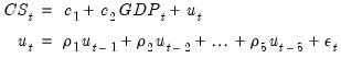
If you wish to estimate a model with autocorrelations from one to five:
 | (24.41) |
you may define your specification using:
cs c gdp ar(1) ar(2) ar(3) ar(4) ar(5)
or more concisely
cs c gdp ar(1 to 5)
The latter form specifies a lag range from 1 to 5 using the to keyword.
We emphasize the fact that you must explicitly list AR lags that you wish to include. By requiring that you enter all of the desired AR terms, EViews allows you the flexibility to restrict lower order correlations to be zero. For example, if you have quarterly data and want only to include a single term to account for seasonal autocorrelation, you could enter
cs c gdp ar(4)
For specifications defined by expression, you must list the coefficient assignment for each of the lags separately, separated by commas:
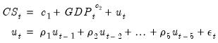 | (24.42) |
you would enter
cs = c(1) + gdp^c(2) + [ar(1)=c(3), ar(2)=c(4), ar(3)=c(5), ar(4)=c(6), ar(5)=c(7)]
Seasonal AR
Seasonal AR terms may be added using the sar keyword, followed by a lag or lag range enclosed in parentheses. The specification
cs c gdp ar(1) sar(4)
will define an AR(5) model with coefficient restrictions as described above (
“Seasonal ARMA Terms”).
Note that in the absence ordinary AR terms, the sar is equivalent to an ar. Thus,
cs c gdp ar(4)
cs c gdp sar(4)
are equivalent specifications.
Specifying MA Terms
To specify an MA term in EViews, you will use the keyword ma, followed by the desired lag or lag range enclosed in parentheses. You must explicitly instruct EViews to use each MA lag you wish to include. You may use the to keyword to define a lag range.
For specifications defined by list,:
 | (24.43) |
you would specify the equation as
cs c gdp ma(1) ma(2)
or more concisely as
cs c gdp ma(1 to 2)
For specifications defined by expression, the MA keywords require coefficient assignments for each lag so that they must be entered individually. Thus, for
 | (24.44) |
you would enter
cs = c(1) + gdp^c(2) + [ma(1)=c(3), ma(2)=c(4)]
Seasonal MA terms may be added using the sma keyword, followed by a lag enclosed in parentheses. The specification
cs c gdp ma(1) ma(4)
will define an MA(5) model with coefficient restrictions as described above (
“Seasonal ARMA Terms”). Note that in the absence of ordinary MA terms, the
sma is equivalent to an
ma. Thus,
cs c gdp ma(4)
cs c gdp sma(4)
are equivalent specifications.
Specifying Differencing
There are two distinct methods of specifying differencing in EViews:
• For integer differencing, you will apply the difference operator to the dependent and explanatory variables either before estimation, or by using series expressions in the equation specification.
• For fractional differencing, you will, include the d keyword in the by-list equation specification to indicate that the dependent and explanatory variables should be fractionally differenced.
Integer Differencing
The d operator may be used to specify integer differences of series. To specify first differencing, simply include the series name in parentheses after d. For example, d(gdp) specifies the first difference of GDP, or GDP–GDP(–1).
Higher-order and seasonal differencing may be specified using the two optional parameters,

and

.
d(x,n) specifies the

-th order difference of the series X:
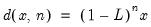 | (24.45) |
where

is the lag operator. For example,
d(gdp,2) specifies the second order difference of GDP:
d(gdp,2) = gdp – 2*gdp(–1) + gdp(–2)
d(x,n,s) specifies

-th order ordinary differencing of X with a multiplicative seasonal difference at lag

:
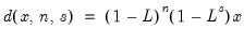 | (24.46) |
For example, d(gdp,0,4) specifies zero ordinary differencing with a seasonal difference at lag 4, or GDP–GDP(–4).
If you need to work in logs, you can also use the
dlog operator, which returns differences in the log values. For example,
dlog(gdp) specifies the first difference of log(GDP) or log(GDP)–log(GDP(–1)). You may also specify the

and

options as described for the simple
d operator,
dlog(x,n,s).
There are two ways to estimate ARIMA models in EViews. First, you may generate a new series containing the differenced data, and then estimate an ARMA model using the new data. For example, to estimate a Box-Jenkins ARIMA(1, 1, 1) model for M1 you can first create the difference series by typing in the command line:
series dm1 = d(m1)
and then use this series when you enter your equation specification:
dm1 c ar(1) ma(1)
Alternatively, you may include the difference operator d directly in the estimation specification. For example, the same ARIMA(1,1,1) model can be estimated using the command:
d(m1) c ar(1) ma(1)
The latter method should generally be employed for an important reason. If you define a new variable, such as DM1 above, and use it in your estimation procedure, then when you forecast from the estimated model, EViews will produce forecasts of the dependent variable DM1. That is, you will get a forecast of the differenced series. If you are really interested in forecasts of the level variable, in this case M1, you will have to manually transform the forecasted value and adjust the computed standard errors accordingly.
Furthermore, if any other transformation or lags of the original series M1 are included as regressors, EViews will not know that they are related to DM1. If, however, you specify the model using the difference operator expression for the dependent variable, d(m1), the forecasting procedure will provide you with the option of forecasting the level variable, in this case M1.
The difference operator may also be used in specifying exogenous variables and can be used in equations with or without ARMA terms. Simply include the series expression in the list of regressors. For example:
d(cs, 2) c d(gdp,2) d(gdp(-1),2) d(gdp(-2),2) time
is a valid specification that employs the difference operator on both the left-hand and right-hand sides of the equation.
Fractional Differencing
If you wish to perform fractional differencing as part of ARFIMA estimation, simply add the d keyword to the existing specification.
Note that fractional integration models may only be estimated in equations specified by list. You may not specify an ARFIMA model using expression.
Specification Examples
For example, to estimate a second-order autoregressive and first-order moving average error process ARMA(2, 1), you would include expressions for the AR(1), AR(2), and MA(1) terms along with the dependent variable (INC) and your other regressors (in this case C and GOV):
inc c gov ar(1 to 2) ma(1)
Once again, you need not use AR and MA terms consecutively. For example, if you want to fit a fourth-order autoregressive model, you could use AR(4) by itself, resulting in a restricted ARMA(4, 0):
inc c gov ar(4)
You may also specify a pure moving average model by using only MA terms. Thus:
inc c gov ma(1) ma(2)
indicates an ARMA(0, 2) model for the errors of the INC equation.
The traditional Box-Jenkins or ARMA models do not have right-hand side variables except for the constant. In this case, your list of regressors would just contain a C in addition to the AR and MA terms. For example:
log(inc) c ar(1) ar(2) ma(1) ma(2)
is a standard Box-Jenkins ARIMA (2, 1, 2) model for log INC.
You may specify an range of MA terms to include using the to keyword. The following ARFIMA(0, 1, 5) specification includes all of the MA terms from 1 to 5, along with the mean regressor DLOG(GDP):
dlog(inc) dlog(cs) c dlog(gdp) ma(1 to 5)
For equations specified by expression, simply enter the explicit equation involving the possibly differenced dependent variable, and add any expressions for AR and MA terms in square brackets:
dlog(cs) = c(1) + dlog(gdp)^c(2) + [ar(1)=c(3), ar(2)=c(4), ma(1)=c(5), ma(2)=c(6)]
To estimate an ARFIMA(2,

, 1) (fractionally integrated second-order autoregressive, first-order moving average error model), you would include expressions for the AR(1), AR(2), and MA(1) terms and the
d keyword along with the dependent variable (INC) and other regressors (C and GOV):
log(inc) c log(gov) ar(1 to 2) ma(1) d
Estimation Options
Clicking on the tab displays a variety of estimation options. The available options will differ depending on whether your equation is specified by list or by expression and whether there are ARMA and fractional differencing components. For the remainder of this discussion, we will assume that you have included ARMA or fractional differencing in the equation specification, and we discuss in turn the settings available for each specification method.
Equations Specified By List
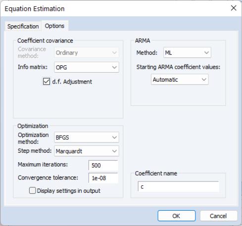
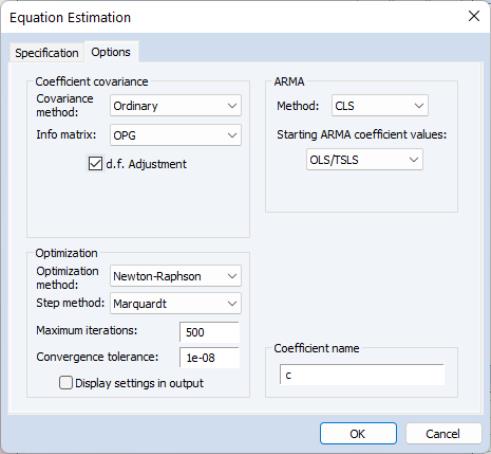
If your equation is specified by list, clicking on the tab displays a dialog page that offers settings for controlling the ARMA estimation, for computing the coefficient covariance, for optimization, and for setting the default coefficient name.
ARMA
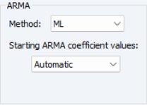
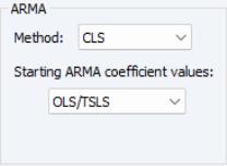
The section of the page controls the method for estimating your ARMA components and setting starting values.
ARMA Method
The dropdown specifies the objective function used in the estimation method:
• For models without fractional differencing, you may choose between the default (maximum likelihood), (generalized least squares), and (conditional least squares) estimation.
• For models with fractional differencing, you may choose between the default and estimation ( is not available for ARFIMA models).
See
“Estimation Method Details” for discussion of these objective functions.
Starting Values
The nonlinear estimation techniques used to estimate ARMA and ARFIMA models require starting values for all coefficient estimates. Normally, EViews determines its own starting values and for the most part this is an issue with which you need not be concerned. There are, however, occasions where you may want to override the default starting values.
First, estimation will sometimes halt when the maximum number of iterations is reached, despite the fact that convergence is not achieved. Resuming the estimation with starting values left over from previous estimation instructs EViews to continue from where it left off instead of starting over. You may also want to try different starting values to ensure that the estimates are a global rather than a local minimum. You might also want to supply starting values if you have a rough idea of what the answers should be, and want to speed up the estimation process.
The dropdown will offer choices for overriding the default EViews starting values. The available starting value options will differ depending on the ARMA method selected above:
• If you select ML or GLS estimation as your method, you will be presented with the choice of , , , and .
For , all of the coefficients are taken from the values in the coefficient vector in the workfile as described below.
For each of the remaining methods, the mean coefficients are obtained from simple OLS regression.
The default EViews initializes the ARMA coefficients using least squares regression of residuals against lagged residuals (for AR terms) and innovations (for MA terms), where innovations are obtained by first regressing residuals against many lags of residuals. sets the ARMA coefficients to arbitrary fixed values of 0.0025 for ordinary ARMA and 0.01 for seasonal ARMA terms. generates randomized ARMA coefficients.
For ARFIMA estimation, the fractional difference parameter is initialized using the Geweke and Porter-Hundlak (1983) log periodogram regression (), a fixed value of 0.1 (), or a randomly generated uniform

().
• If you select the estimation method, the starting values dropdown will let you choose between , ., ., , and .
For the selection, all of the coefficients are initialized from the values in the coefficient vector in the workfile as described below.
For the variants of , EViews will initialize the mean coefficients at the specified fraction of the simple OLS or TSLS estimates while sets the mean coefficients to zero.
Coefficients for ARMA terms are always set to arbitrary fixed values of 0.0025 for ordinary ARMA and 0.01 for seasonal ARMA terms.
For you to usefully set user-specified starting values, you will need a little more information about how EViews assigns coefficients for the ARMA terms.
EViews assigns coefficient numbers to the variables in the following order:
• First are the coefficients of the variables, in order of entry.
• Next is the ARFIMA coefficient.
• Next come the AR terms in the order of entry.
• The SAR, MA, and SMA coefficients follow, in that order.
(Following estimation, you can always see the assignment of coefficients by looking at the view of your equation.)
Thus the following two specifications will have their coefficients in the same order:
y c x ma(2) ma(1) sma(4) ar(1)
y sma(4) c ar(1) ma(2) x ma(1)
By default EViews uses the built-in C coefficient vector, but this may be overridden (see
“Coefficient Name”). To set initial values, you may edit the corresponding elements of the coefficient vector in the workfile, or you may also assign values in the vector using the
param command:
param c(1) 50 c(2) .8 c(3) .2 c(4) .6 c(5) .1 c(6) .5
The starting values will be 50 for the constant, 0.8 for X, 0.2 for AR(1), 0.6 for MA(2), 0.1 for MA(1) and 0.5 for SMA(4).
Backcasting
If your specification includes MA terms and the ARMA estimation method is CLS, EViews will display a checkbox for whether or not to use backcasting to initialize the MA innovations. By default, EViews performs backcasting as described in
“Initializing MA Innovations”, but you can unselect this option to set the presample innovations to their unconditional expectation of zero.
Coefficient Covariance
The section of the page controls the computation of the estimates of the precision of your coefficient estimates.
The options that are available will depend on the ARMA estimation method.
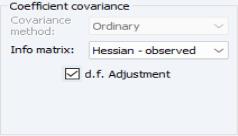
• For ML or GLS estimation, covariances are always calculated by taking the inverse of the an estimate of the information matrix.
The default setting for estimation uses the outer product of the gradients (), but you may instead use the dropdown to use the observed Hessian ().
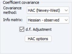
• For estimation, you may choose a using the dropdown menu.
The default method takes the inverse of the estimate of the information matrix. Alternately you may choose to compute or sandwich covariances.
In the latter case, EViews will display a button which you may use to access various settings for controlling the long-run covariance estimation.
The dropdown menu will offer you the choice between computing the information matrix estimate using the outer product of the gradients () or the observed Hessian ().
If you select GLS or CLS estimation, the covariance matrix will, by default, employ a degree-of-freedom correction. If you select ML estimation the default computation will not employ degree-of-freedom correction. In all three cases, the checkbox may be used to modify the computation.
Estimation Algorithm
EViews provides a number of options that allow you to control the iterative procedure of the estimation algorithm. In general, you can rely on the EViews choices, but on occasion you may wish to override the default settings.
The section of the dialog contains settings for the numeric optimization of your likelihood or least squares objective function.
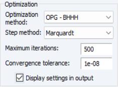
By default, EViews estimates ARMA and ARFIMA models using the Broyden, Fletcher, Goldfarb and Shanno (BFGS) algorithm. You may use the dropdown to select a different method:
• For models estimated using ML and GLS, you may choose to estimate your model using , (Gauss-Newton using the outer-product of the gradient), (transformation to pseudo-GLS regression model), and .
• For models estimated using CLS, you may choose between , , , and The latter employs OPG/BHHH with a Marquardt diagonal adjustment.
• For all but EViews, the combo lets you choose between the default , , and determined steps. The default method is .
In addition, you can use the and edit fields to change the stopping rules from their global default settings. Checking the in output box instructs EViews to put information about starting values and other optimization settings at the top of your equation output.
Coefficient Name
For equations specified by list EViews will, by default, use the built-in C vector to hold coefficient estimates. You may change this assignment by entering the name of a coefficient object in the edit field.
If the coefficient does not exist, EViews will create it and size it appropriately. If the coefficient already exists, it will be resized if necessary so that it is large enough to hold the results. If an object of a different type with that name is present in the workfile, EViews will issue an error message.
Equation Specified By Expression
If your equation is specified by expression, clicking on the tab displays a dialog page that offers a subset of the settings that are available for equations specified by list.
You may use the page to control the computation of the coefficient covariance, the optimization method, the ARMA starting coefficient values, and the default coefficient name.
Coefficient Covariance
The section of the page allows you to specify a using the dropdown menu. You may choose to compute the default , or the , or sandwich covariances. If you select , EViews will display a button which you may use to access various settings for controlling the long-run covariance estimation.
As before, the dropdown menu will offer you the choice between computing the information matrix estimate using the outer product of the gradients () or the observed Hessian ().
By default, EViews will apply a degree-of-freedom correction to the estimated covariance matrix. You may uncheck the checkbox to remove this correction.
Estimation Algorithm
By default, EViews estimates by-expression ARMA and ARFIMA models using . You may use the dropdown to choose between , , , and the latter of which employs Gauss-Newton with a Marquardt diagonal adjustment.
Where appropriate, the combo lets you choose between the default , , and determined steps.
The and edit fields may be used to limit the number of iterations and to set the algorithm stopping rule. Checking the in output box instructs EViews to put information about starting values and other optimization settings at the top of your equation output.
ARMA Method
You will not be able to specify an ARMA method as ARMA equations specified by expression may only use the CLS objective.
Starting Values
The starting value dropdown menu lets you choose between the default and , ., ., , and .
For the variants of , EViews will initialize the mean coefficients at the specified fraction of the simple OLS or TSLS estimates (ignoring ARMA terms), while sets the mean coefficients to zero. Coefficients for ARMA terms are always set to arbitrary fixed values of 0.0025 for ordinary ARMA and 0.01 for seasonal ARMA terms.
For the selection, the coefficients are initialized from the values in the coefficient vector in the workfile.