Testing for Serial Correlation
Before you use an estimated equation for statistical inference (e.g. hypothesis tests and forecasting), you should generally examine the residuals for evidence of serial correlation. EViews provides several methods of testing a specification for the presence of serial correlation.
The Durbin-Watson Statistic
EViews reports the Durbin-Watson (DW) statistic as a part of the standard regression output. The Durbin-Watson statistic is a test for first-order serial correlation. More formally, the DW statistic measures the linear association between adjacent residuals from a regression model. The Durbin-Watson is a test of the hypothesis

in the specification:
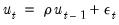 | (24.38) |
If there is no serial correlation, the DW statistic will be around 2. The DW statistic will fall below 2 if there is positive serial correlation (in the worst case, it will be near zero). If there is negative correlation, the statistic will lie somewhere between 2 and 4.
Positive serial correlation is the most commonly observed form of dependence. As a rule of thumb, with 50 or more observations and only a few independent variables, a DW statistic below about 1.5 is a strong indication of positive first order serial correlation. See Johnston and DiNardo (1997, Chapter 6.6.1) for a thorough discussion on the Durbin-Watson test and a table of the significance points of the statistic.
There are three main limitations of the DW test as a test for serial correlation. First, the distribution of the DW statistic under the null hypothesis depends on the data matrix

. The usual approach to handling this problem is to place bounds on the critical region, creating a region where the test results are inconclusive. Second, if there are lagged dependent variables on the right-hand side of the regression, the DW test is no longer valid. Lastly, you may only test the null hypothesis of no serial correlation against the alternative hypothesis of first-order serial correlation.
Two other tests of serial correlation—the Q-statistic and the Breusch-Godfrey LM test—overcome these limitations, and are preferred in most applications.
Correlograms and Q-statistics
If you selecton the equation toolbar, EViews will display the autocorrelation and partial autocorrelation functions of the residuals, together with the Ljung-Box Q-statistics for high-order serial correlation. If there is no serial correlation in the residuals, the autocorrelations and partial autocorrelations at all lags should be nearly zero, and all Q-statistics should be insignificant with large p-values.
Note that the p-values of the Q-statistics will be computed with the degrees of freedom adjusted for the inclusion of ARMA terms in your regression. There is evidence that some care should be taken in interpreting the results of a Ljung-Box test applied to the residuals from an ARMAX specification (see Dezhbaksh, 1990, for simulation evidence on the finite sample performance of the test in this setting).
Details on the computation of correlograms and
Q-statistics are provided in greater detail in
“Series” .
Serial Correlation LM Test
Selecting carries out the Breusch-Godfrey Lagrange multiplier test for general, high-order, ARMA errors. In the dialog box, you should enter the highest order of serial correlation to be tested.
The null hypothesis of the test is that there is no serial correlation in the residuals up to the specified order. EViews reports a statistic labeled “
F-statistic” and an “Obs*R-squared” (

—the number of observations times the R-square) statistic. The

statistic has an asymptotic

distribution under the null hypothesis. The distribution of the
F-statistic is not known, but is often used to conduct an informal test of the null.
See
“Serial Correlation LM Test” for further discussion of the serial correlation LM test.
Example
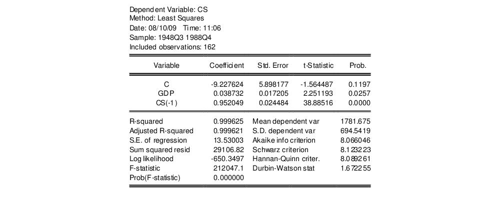
As an example of the application of serial correlation testing procedures, consider the following results from estimating a simple consumption function by ordinary least squares using data in the workfile “Uroot.WF1”:
A quick glance at the results reveals that the coefficients are statistically significant and the fit is very tight. However, if the error term is serially correlated, the estimated OLS standard errors are invalid and the estimated coefficients will be biased and inconsistent due to the presence of a lagged dependent variable on the right-hand side. The Durbin-Watson statistic is not appropriate as a test for serial correlation in this case, since there is a lagged dependent variable on the right-hand side of the equation.
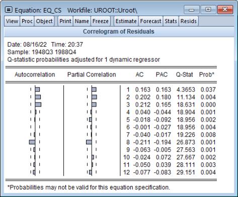
Selecting for the first 12 lags from this equation produces the following view:
The correlogram has spikes at lags up to three and at lag eight. The Q-statistics are significant at all lags, indicating significant serial correlation in the residuals.
Selecting and entering a lag of 4 yields the following result (top portion only):
The test rejects the hypothesis of no serial correlation up to order four. The Q-statistic and the LM test both indicate that the residuals are serially correlated and the equation should be re-specified before using it for hypothesis tests and forecasting.