Forecast Basics
EViews stores the forecast results in the series specified in the Forecast name field. We will refer to this series as the forecast series.
The
forecast sample specifies the observations for which EViews will try to compute fitted or forecasted values. If the forecast is not computable, a missing value will be returned. In some cases, EViews will carry out automatic adjustment of the sample to prevent a forecast consisting entirely of missing values (see
“Adjustment for Missing Values”, below). Note that the forecast sample may or may not overlap with the sample of observations used to estimate the equation.
For values not included in the forecast sample, there are two options. By default, EViews fills in the actual values of the dependent variable. If you turn off the option, out-of-forecast-sample values will be filled with NAs.
As a consequence of these rules, all data in the forecast series will be overwritten during the forecast procedure. Existing values in the forecast series will be lost.
Computing Point Forecasts
For each observation in the forecast sample, EViews computes the fitted value of the dependent variable using the estimated parameters, the right-hand side exogenous variables, and either the actual or estimated values for lagged endogenous variables and residuals. The method of constructing these forecasted values depends upon the estimated model and user-specified settings.
To illustrate the forecasting procedure, we begin with a simple linear regression model with no lagged endogenous right-hand side variables, and no ARMA terms. Suppose that you have estimated the following equation specification:
y c x z
Now click on , specify a forecast period, and click OK.
For every observation in the forecast period, EViews will compute the fitted value of Y using the estimated parameters and the corresponding values of the regressors, X and Z:
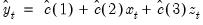 | (25.1) |
You should make certain that you have valid values for the exogenous right-hand side variables for all observations in the forecast period. If any data are missing in the forecast sample, the corresponding forecast observation will be an NA.
Adjustment for Missing Values
There are two cases when a missing value will be returned for the forecast value. First, if any of the regressors have a missing value, and second, if any of the regressors are out of the range of the workfile. This includes the implicit error terms in AR models.
In the case of forecasts with no dynamic components in the specification (i.e. with no lagged endogenous or ARMA error terms), a missing value in the forecast series will not affect subsequent forecasted values. In the case where there are dynamic components, however, a single missing value in the forecasted series will propagate throughout all future values of the series.
As a convenience feature, EViews will move the starting point of the sample forward where necessary until a valid forecast value is obtained. Without these adjustments, the user would have to figure out the appropriate number of presample values to skip, otherwise the forecast would consist entirely of missing values. For example, suppose you wanted to forecast dynamically from the following equation specification:
y c y(-1) ar(1)
If you specified the beginning of the forecast sample to the beginning of the workfile range, EViews will adjust forward the forecast sample by 2 observations, and will use the pre-forecast-sample values of the lagged variables (the loss of 2 observations occurs because the residual loses one observation due to the lagged endogenous variable so that the forecast for the error term can begin only from the third observation.)
Forecast Errors and Variances
Suppose the “true” model is given by:
 | (25.2) |
where

is an independent, and identically distributed, mean zero random disturbance, and

is a vector of unknown parameters. Below, we relax the restriction that the

’s be independent.
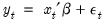
The true model generating

is not known, but we obtain estimates

of the unknown parameters

. Then, setting the error term equal to its mean value of zero, the (point) forecasts of

are obtained as:
 | (25.3) |
Forecasts are made with error, where the error is simply the difference between the actual and forecasted value
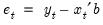
. Assuming that the model is correctly specified, there are two sources of forecast error: residual uncertainty and coefficient uncertainty.
Residual Uncertainty
The first source of error, termed
residual or
innovation uncertainty, arises because the innovations

in the equation are unknown for the forecast period and are replaced with their expectations. While the residuals are zero in expected value, the individual values are non-zero; the larger the variation in the individual residuals, the greater the overall error in the forecasts.
The standard measure of this variation is the standard error of the regression (labeled “S.E. of regression” in the equation output). Residual uncertainty is usually the largest source of forecast error.
In dynamic forecasts, innovation uncertainty is compounded by the fact that lagged dependent variables and ARMA terms depend on lagged innovations. EViews also sets these equal to their expected values, which differ randomly from realized values. This additional source of forecast uncertainty tends to rise over the forecast horizon, leading to a pattern of increasing forecast errors. Forecasting with lagged dependent variables and ARMA terms is discussed in more detail below.
Coefficient Uncertainty
The second source of forecast error is
coefficient uncertainty. The estimated coefficients

of the equation deviate from the true coefficients

in a random fashion. The standard error of the estimated coefficient, given in the regression output, is a measure of the precision with which the estimated coefficients measure the true coefficients.
The effect of coefficient uncertainty depends upon the exogenous variables. Since the estimated coefficients are multiplied by the exogenous variables

in the computation of forecasts, the more the exogenous variables deviate from their mean values, the greater is the forecast uncertainty.
Forecast Variability
The variability of forecasts is measured by the forecast standard errors. For a single equation without lagged dependent variables or ARMA terms, the forecast standard errors are computed as:
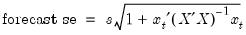 | (25.4) |
where

is the standard error of regression. These standard errors account for both innovation (the first term) and coefficient uncertainty (the second term). Point forecasts made from linear regression models estimated by least squares are optimal in the sense that they have the smallest forecast variance among forecasts made by linear unbiased estimators. Moreover, if the innovations are normally distributed, the forecast errors have a
t-distribution and forecast intervals can be readily formed.
If you supply a name for the forecast standard errors, EViews computes and saves a series of forecast standard errors in your workfile. You can use these standard errors to form forecast intervals. If you choose the Do graph option for output, EViews will plot the forecasts with plus and minus two standard error bands. These two standard error bands provide an approximate 95% forecast interval; if you (hypothetically) make many forecasts, the actual value of the dependent variable will fall inside these bounds 95 percent of the time.
Additional Details
EViews accounts for the additional forecast uncertainty generated when lagged dependent variables are used as explanatory variables (see
“Forecasts with Lagged Dependent Variables”).
There are cases where coefficient uncertainty is ignored in forming the forecast standard error. For example, coefficient uncertainty is always ignored in equations specified by expression, for example, nonlinear least squares, and equations that include PDL (polynomial distributed lag) terms (
“Forecasting with Nonlinear and PDL Specifications”).
In addition, forecast standard errors do not account for GLS weights in estimated panel equations.
Forecast Evaluation
Suppose we construct a dynamic forecast for HS over the period 1990M02 to 1996M01 using our estimated housing equation. If the Forecast evaluation option is checked, and there are actual data for the forecasted variable for the forecast sample, EViews reports a table of statistical results evaluating the forecast:
Note that EViews cannot compute a forecast evaluation if there are no data for the dependent variable for the forecast sample.
The forecast evaluation is saved in one of two formats. If you turn on the Do graph option, the forecasts are included along with a graph of the forecasts. If you wish to display the evaluations in their own table, you should turn off the Do graph option in the Forecast dialog box.
Suppose the forecast sample is
, and denote the actual and forecasted value in period

as

and

, respectively. The reported forecast error statistics are computed as follows:
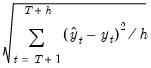
Root Mean Squared Error | |
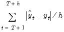
Mean Absolute Error | |
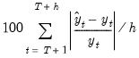
Mean Absolute Percentage Error | |
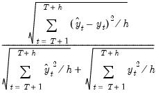
Theil Inequality Coefficient | |
The first two forecast error statistics depend on the scale of the dependent variable. These should be used as relative measures to compare forecasts for the same series across different models; the smaller the error, the better the forecasting ability of that model according to that criterion. The remaining two statistics are scale invariant. The Theil inequality coefficient always lies between zero and one, where zero indicates a perfect fit.
The mean squared forecast error can be decomposed as:
 | (25.5) |
where

,

,

,

are the means and (biased) standard deviations of

and

, and

is the correlation between

and

. The proportions are defined as:
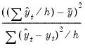
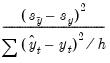
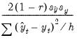
Bias Proportion | |
Variance Proportion | |
Covariance Proportion | |
• The bias proportion tells us how far the mean of the forecast is from the mean of the actual series.
• The variance proportion tells us how far the variation of the forecast is from the variation of the actual series.
• The covariance proportion measures the remaining unsystematic forecasting errors.
Note that the bias, variance, and covariance proportions add up to one.
If your forecast is “good”, the bias and variance proportions should be small so that most of the bias should be concentrated on the covariance proportions. For additional discussion of forecast evaluation, see Pindyck and Rubinfeld (1998, p. 210-214).
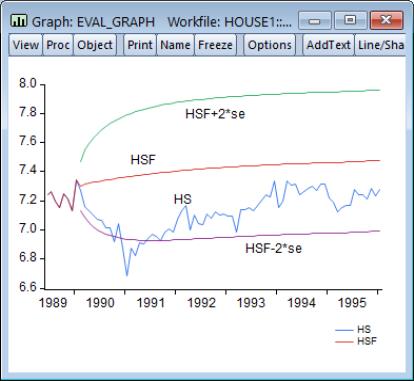
For the example output, the bias proportion is large, indicating that the mean of the forecasts does a poor job of tracking the mean of the dependent variable. To check this, we will plot the forecasted series together with the actual series in the forecast sample with the two standard error bounds. Suppose we saved the forecasts and their standard errors as HSF and HSFSE, respectively. Then the plus and minus two standard error series can be generated by the commands:
smpl 1990m02 1996m01
series hsf_high = hsf + 2*hsfse
series hsf_low = hsf - 2*hsfse
Create a group containing the four series. You can highlight the four series HS, HSF, HSF_HIGH, and HSF_LOW, double click on the selected area, and select , or you can select and enter the four series names. Once you have the group open, select and select Line & Symbolfrom the left side of the dialog.
The forecasts completely miss the downturn at the start of the 1990’s, but, subsequent to the recovery, track the trend reasonably well from 1992 to 1996.