Vector Error Correction (VEC) Models
A vector error correction (VEC) model is a restricted VAR designed for use with nonstationary series that are known to be cointegrated. You may test for cointegration using an estimated VAR object, Equation object estimated using nonstationary regression methods, or using a Group object (see
“Cointegration Testing”).
The VEC has cointegration relations built into the specification so that it restricts the long-run behavior of the endogenous variables to converge to their cointegrating relationships while allowing for short-run adjustment dynamics. The cointegration term is known as the error correction term since the deviation from long-run equilibrium is corrected gradually through a series of partial short-run adjustments.
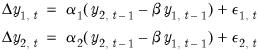
To take the simplest possible example, consider a two variable system with one cointegrating equation and no lagged difference terms. The cointegrating equation is:
 | (44.39) |
The corresponding VEC model is:
 | (44.40) |
In this simple model, the only right-hand side variable is the error correction term. In long run equilibrium, this term is zero. However, if

and

deviate from the long run equilibrium, the error correction term will be nonzero and each variable adjusts to partially restore the equilibrium relation. The coefficient

measures the speed of adjustment of the
i-th endogenous variable towards the equilibrium.
How to Estimate a VEC
As the VEC specification only applies to cointegrated series, you should first run the Johansen cointegration test as described above and determine the number of cointegrating relations. You will need to provide this information as part of the VEC specification.
To set up a VEC, click the button in the VAR toolbar and choose the Vector Error Correction specification from the VAR/VEC Specification tab. In the VAR/VEC Specification tab, you should provide the same information as for an unrestricted VAR, except that:
• The constant or linear trend term should not be included in the Exogenous Series edit box. The constant and trend specification for VECs should be specified in the Cointegration tab (see below).
• The lag interval specification refers to lags of the first difference terms in the VEC. For example, the lag specification “1 1” will include lagged first difference terms on the right-hand side of the VEC. Rewritten in levels, this VEC is a restricted VAR with two lags. To estimate a VEC with no lagged first difference terms, specify the lag as “0 0”.
• The constant and trend specification for VECs should be specified in the
Cointegration tab. You must choose from one of the five Johansen (1995) trend specifications as explained in
“Deterministic Trend Specification”. You must also specify the number of cointegrating relations in the appropriate edit field. This number should be a positive integer less than the number of endogenous variables in the VEC.
• If you want to impose restrictions on the cointegrating relations and/or the adjustment coefficients, use the
Restrictions tab.
“Imposing VEC Restrictions” describes these restriction in greater detail. Note that the contents of this tab are grayed out unless you have clicked the
Vector Error Correction specification in the
VAR/VEC Specification tab.
Once you have filled the dialog, simply click OK to estimate the VEC. Estimation of a VEC model is carried out in two steps. In the first step, we estimate the cointegrating relations from the Johansen procedure as used in the cointegration test. We then construct the error correction terms from the estimated cointegrating relations and estimate a VAR in first differences including the error correction terms as regressors.
VEC Estimation Output
The VEC estimation output consists of two parts. The first part reports the results from the first step Johansen procedure. If you did not impose restrictions, EViews will use a default normalization that identifies all cointegrating relations. This default normalization expresses the first

variables in the VEC as functions of the remaining

variables, where

is the number of cointegrating relations and

is the number of endogenous variables. Asymptotic standard errors (corrected for degrees of freedom) are reported for parameters that are identified under the restrictions. If you provided your own restrictions, standard errors will not be reported unless the restrictions identify all cointegrating vectors.
The second part of the output reports results from the second step VAR in first differences, including the error correction terms estimated from the first step. The error correction terms are denoted
CointEq1,
CointEq2, and so on in the output. This part of the output has the same format as the output from unrestricted VARs as explained in
“Estimation Output”, with one difference. At the bottom of the VEC output table, you will see two log likelihood values reported for the system. The first value, labeled
Log Likelihood (d.f. adjusted), is computed using the determinant of the residual covariance matrix (reported as
Determinant Residual Covariance), using small sample degrees of freedom correction as in
(44.11). This is the log likelihood value reported for unrestricted VARs. The
Log Likelihood value is computed using the residual covariance matrix without correcting for degrees of freedom. This log likelihood value is comparable to the one reported in the cointegration test output.
Views and Procs of a VEC
Views and procs available for VECs are mostly the same as those available for VARs as explained above. Here, we only mention those that are specific to VECs.
Cointegrating Relations
displays a graph of the estimated cointegrating relations as used in the VEC. To store these estimated cointegrating relations as named series in the workfile, use . This proc will create and display an untitled group object containing the estimated cointegrating relations as named series. These series are named COINTEQ01, COINTEQ02 and so on.
Forecasting
To forecast from your VEC, click on the Forecast button on the toolbar and fill out the dialog as described in
“Forecasting”Data Members
Various results from the estimated VAR/VEC can be retrieved through the command line data members.
“Var Data Members” provides a complete list of data members that are available for a VAR object. Here, we focus on retrieving the estimated coefficients of a VAR/VEC.
Obtaining Coefficients of a VAR
Coefficients of (unrestricted) VARs can be accessed by referring to elements of a two dimensional array C. The first dimension of C refers to the equation number of the VAR, while the second dimension refers to the variable number in each equation. For example, C(2,3) is the coefficient of the third regressor in the second equation of the VAR. The C(2,3) coefficient of a VAR named VAR01 can then be accessed by the command
var01.c(2,3)
To examine the correspondence between each element of C and the estimated coefficients, select from the VAR toolbar.
Obtaining Coefficients of a VEC
For VEC models, the estimated coefficients are stored in three different two dimensional arrays: A, B, and C. A contains the adjustment parameters

, B contains the cointegrating vectors

, and C holds the short-run parameters (the coefficients on the lagged first difference terms).
• The first index of A is the equation number of the VEC, while the second index is the number of the cointegrating equation. For example, A(2,1) is the adjustment coefficient of the first cointegrating equation in the second equation of the VEC.
• The first index of B is the number of the cointegrating equation, while the second index is the variable number in the cointegrating equation. For example, B(2,1) is the coefficient of the first variable in the second cointegrating equation. Note that this indexing scheme corresponds to the
transpose of

.
• The first index of C is the equation number of the VEC, while the second index is the variable number of the first differenced regressor of the VEC. For example, C(2, 1) is the coefficient of the first differenced regressor in the second equation of the VEC.
You can access each element of these coefficients by referring to the name of the VEC followed by a dot and coefficient element:
var01.a(2,1)
var01.b(2,1)
var01.c(2,1)
To see the correspondence between each element of A, B, and C and the estimated coefficients, select from the VAR toolbar.
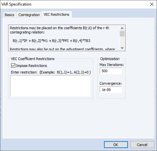
Imposing VEC Restrictions
Since the cointegrating vector

is not fully identified, you may wish to impose your own identifying restrictions when performing estimation.
Restrictions can be imposed on the cointegrating vector (elements of the

matrix) and/or on the adjustment coefficients (elements of the

matrix). To impose restrictions in estimation, open the test, select in the main VAR estimation dialog, then click on the tab. You will enter your restrictions in the edit box that appears when you check the box:
Restrictions on the Cointegrating Vector
To impose restrictions on the cointegrating vector

, you must refer to the (
i,
j)-th element of the
transpose of the

matrix by
B(i,j). The
i-th cointegrating relation has the representation:
B(i,1)*y1 + B(i,2)*y2 + ... + B(i,k)*yk
where y1, y2, ... are the (lagged) endogenous variable. Then, if you want to impose the restriction that the coefficient on y1 for the second cointegrating equation is 1, you would type the following in the edit box:
B(2,1) = 1
You can impose multiple restrictions by separating each restriction with a comma on the same line or typing each restriction on a separate line. For example, if you want to impose the restriction that the coefficients on y1 for the first and second cointegrating equations are 1, you would type:
B(1,1) = 1
B(2,1) = 1
Currently
all restrictions must be linear (or more precisely affine) in the elements of the  matrix
. So for example
B(1,1) * B(2,1) = 1
will return a syntax error.
Restrictions on the Adjustment Coefficients
To impose restrictions on the adjustment coefficients, you must refer to the (
i,
j)-th elements of the

matrix by
A(i,j). The error correction terms in the
i-th VEC equation will have the representation:
A(i,1)*CointEq1 + A(i,2)*CointEq2 + ... + A(i,r)*CointEqr
Restrictions on the adjustment coefficients are currently limited to linear homogeneous restrictions so that you must be able to write your restriction as
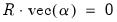
, where

is a known

matrix. This condition implies, for example, that the restriction,
A(1,1) = A(2,1)
is valid but:
A(1,1) = 1
will return a restriction syntax error.
One restriction of particular interest is whether the
i-th row of the

matrix is all zero. If this is the case, then the
i-th endogenous variable is said to be
weakly exogenous with respect to the  parameters
. See Johansen (1995) for the definition and implications of weak exogeneity. For example, if we assume that there is only one cointegrating relation in the VEC, to test whether the second endogenous variable is weakly exogenous with respect to

you would enter:
A(2,1) = 0
To impose multiple restrictions, you may either separate each restriction with a comma on the same line or type each restriction on a separate line. For example, to test whether the second endogenous variable is weakly exogenous with respect to

in a VEC with two cointegrating relations, you can type:
A(2,1) = 0
A(2,2) = 0
You may also impose restrictions on both
 and
and 
. However, the restrictions on

and

must be
independent. So for example,
A(1,1) = 0
B(1,1) = 1
is a valid restriction but:
A(1,1) = B(1,1)
will return a restriction syntax error.
Identifying Restrictions and Binding Restrictions
EViews will check to see whether the restrictions you provided identify all cointegrating vectors for each possible rank. The identification condition is checked numerically by the rank of the appropriate Jacobian matrix; see Boswijk (1995) for the technical details. Asymptotic standard errors for the estimated cointegrating parameters will be reported only if the restrictions identify the cointegrating vectors.
If the restrictions are binding, EViews will report the LR statistic to test the binding restrictions. The LR statistic is reported if the degrees of freedom of the asymptotic

-distribution is positive. Note that the restrictions can be binding even if they are not identifying, (
e.g. when you impose restrictions on the adjustment coefficients but not on the cointegrating vector).
Options for Restricted Estimation
Estimation of the restricted cointegrating vectors

and adjustment coefficients

generally involves an iterative process. The tab provides iteration control for the maximum number of iterations and the convergence criterion. EViews estimates the restricted

and

using the switching algorithm as described in Boswijk (1995). Each step of the algorithm is guaranteed to increase the likelihood and the algorithm should eventually converge (though convergence may be to a local rather than a global optimum). You may need to increase the number of iterations in case you are having difficulty achieving convergence at the default settings.
Once you have filled the dialog, simply click OK to estimate the VEC. Estimation of a VEC model is carried out in two steps. In the first step, we estimate the cointegrating relations from the Johansen procedure as used in the cointegration test. We then construct the error correction terms from the estimated cointegrating relations and estimate a VAR in first differences including the error correction terms as regressors.