Basic ARCH Specifications
In developing an ARCH model, you will have to provide three distinct specifications—one for the conditional mean equation, one for the conditional variance, and one for the conditional error distribution. We begin by describing some basic specifications for these terms. The discussion of more complicated models is taken up in
“Additional ARCH Models”.
The GARCH(1, 1) Model
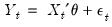
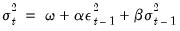
We begin with the simplest GARCH(1,1) specification:
 | (27.1) |
 | (27.2) |
in which the mean equation given in
(27.1) is written as a function of exogenous variables with an error term. Since

is the one-period ahead forecast variance based on past information, it is called the
conditional variance. The conditional variance equation specified in
(27.2) is a function of three terms:
• A constant term:

.
• News about volatility from the previous period, measured as the lag of the squared residual from the mean equation:

(the ARCH term).
• Last period’s forecast variance:

(the GARCH term).
The (1, 1) in GARCH(1, 1) refers to the presence of a first-order autoregressive GARCH term (the first term in parentheses) and a first-order moving average ARCH term (the second term in parentheses). An ordinary ARCH model is a special case of a GARCH specification in which there are no lagged forecast variances in the conditional variance equation—i.e., a GARCH(0, 1).
This specification is often interpreted in a financial context, where an agent or trader predicts this period’s variance by forming a weighted average of a long term average (the constant), the forecasted variance from last period (the GARCH term), and information about volatility observed in the previous period (the ARCH term). If the asset return was unexpectedly large in either the upward or the downward direction, then the trader will increase the estimate of the variance for the next period. This model is also consistent with the volatility clustering often seen in financial returns data, where large changes in returns are likely to be followed by further large changes.
There are two equivalent representations of the variance equation that may aid you in interpreting the model:
• If we recursively substitute for the lagged variance on the right-hand side of
Equation (27.2), we can express the conditional variance as a weighted average of all of the lagged squared residuals:
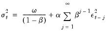 | (27.3) |
We see that the GARCH(1,1) variance specification is analogous to the sample variance, but that it down-weights more distant lagged squared errors.
• The error in the squared returns is given by

. Substituting for the variances in the variance equation and rearranging terms we can write our model in terms of the errors:
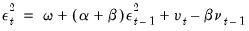 | (27.4) |
Thus, the squared errors follow a heteroskedastic ARMA(1,1) process. The autoregressive root which governs the persistence of volatility shocks is the sum of

plus

. In many applied settings, this root is very close to unity so that shocks die out rather slowly.
The GARCH(q, p) Model
Higher order GARCH models, denoted GARCH(

), can be estimated by choosing either

or

greater than 1 where

is the order of the autoregressive GARCH terms and

is the order of the moving average ARCH terms.
The representation of the GARCH(

) variance is:
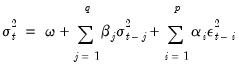 | (27.5) |
The GARCH-M Model
The

in equation
Equation (27.2) represent exogenous or predetermined variables that are included in the mean equation. If we introduce the conditional variance or standard deviation into the mean equation, we get the GARCH-in-Mean (GARCH-M) model (Engle, Lilien and Robins, 1987):
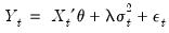 | (27.6) |
The ARCH-M model is often used in financial applications where the expected return on an asset is related to the expected asset risk. The estimated coefficient on the expected risk is a measure of the risk-return tradeoff.
Two variants of this ARCH-M specification use the conditional standard deviation or the log of the conditional variance in place of the variance in
Equation (27.6).
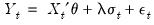 | (27.7) |
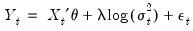 | (27.8) |
Regressors in the Variance Equation
Equation
(27.5) may be extended to allow for the inclusion of exogenous or predetermined regressors,

, in the variance equation:
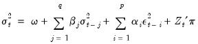 | (27.9) |
Note that the forecasted variances from this model are not guaranteed to be positive. You may wish to introduce regressors in a form where they are always positive to minimize the possibility that a single, large negative value generates a negative forecasted value.
Distributional Assumptions
To complete the basic ARCH specification, we require an assumption about the conditional distribution of the error term

. There are three assumptions commonly employed when working with ARCH models: normal (Gaussian) distribution, Student’s
t-distribution, and the Generalized Error Distribution (GED). Given a distributional assumption, ARCH models are typically estimated by the method of maximum likelihood.
For example, for the GARCH(1, 1) model with conditionally normal errors, the contribution to the log-likelihood for observation

is:
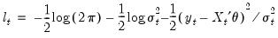 | (27.10) |
where

is specified in one of the forms above.
For the Student’s t-distribution, the log-likelihood contributions are of the form:
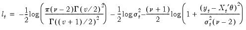 | (27.11) |
where the degree of freedom

controls the tail behavior. The
t-distribution approaches the normal as

.
For the GED, we have:
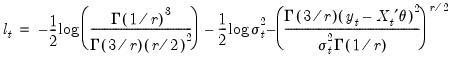 | (27.12) |
where the tail parameter

. The GED is a normal distribution if

, and fat-tailed if

.
By default, ARCH models in EViews are estimated by the method of maximum likelihood under the assumption that the errors are conditionally normally distributed.