Breakpoint Regression in EViews 8
The standard linear regression model assumes that the parameters of the model do not vary across observations. Despite this assumption. structural change, the changing of parameters at dates in the sample period, plays an empirically relevant role in applied time series analysis. Accordingly, there has been a large volume of work targeted at developing testing and estimation methodologies for regression models which allow for change.
EViews 8 introduces tools for estimating linear regression models that are subject to structural change. The regime breakpoints may be known and specified a priori, or they may be estimated using the Bai (1997), Bai and Perron (1998), and related techniques.
You may estimate “pure” breakpoint specifications in which all of the regressors have regime specific coefficients, or specifications in which only some coefficients vary with the regime.
Note that breakpoint regression is closely related to multiple breakpoint testing.
Breakpoint Example
To illustrate the use of these tools in practice, we employ the simple model of the U.S. expost real interest rate from Garcia and Perron (1996) that is used as an example by Bai and Perron (2003 “Computation and Analysis of Multiple Structural Change Models,” Journal of Applied Econometrics, 6, 72–78.). The data, which consist of observations for the three-month treasury rate deflated by the CPI for the period 1961q1–1983q3, are provided in the series RATES in the workfile realrate.wf1.
View a view of this Bai-Perron breakpoint example.
Select Object/New Object.../Equation or Quick/Estimate Equation… from the main menu or enter the command breakls in the command line and hit Enter.
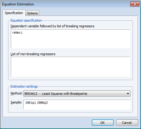
The regression model consists of a regime-specific constant regressor so we enter the dependent variable RATES and C in the topmost edit field. The sample is set to the full workfile range.
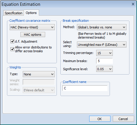
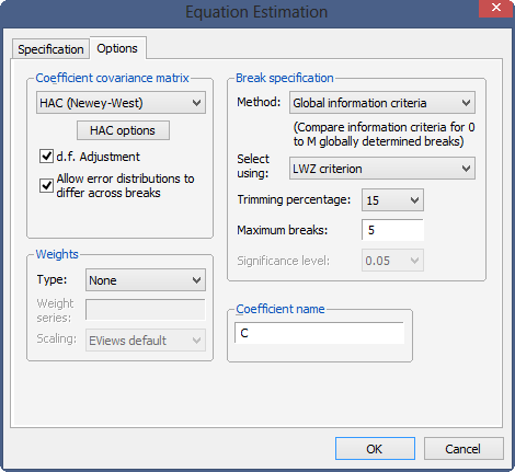
Next, click on the Options tab and specify HAC (Newey-West) standard errors, check Allow error distributions to differ across breaks, choose the Bai-Perron Global L breaks vs. none method using the Unweighted-Max F (UDMax) test to determine the number of breaks, and set a Trimming percentage of 15, and a Significance level of 0.05.
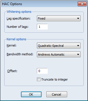
Lastly, to match the test example in Bai and Perron (2003), we click on the HAC Options button and set the options to use a Quadratic-Spectral kernel with Andrews automatic bandwidth and single pre-whitening lag:
Click OK twice to accept the settings and estimate the model. EViews displays the results of the breakpoint selection and coefficient estimation:
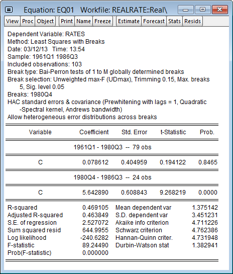
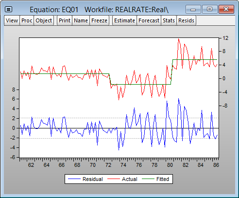
The UDMax methodology selects a single statistically significant break at 1980Q4. The results clearly show a significant difference in the mean RATES prior to and after 1980Q4. Click on View/Actual, Fitted, Residual/Actual, Fitted, Residual Graph, to see in-sample fitted data alongside the original series and the residuals:
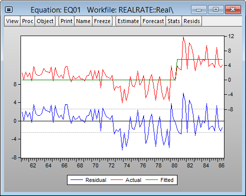
Casual inspection of the residuals suggests that the model might be improved with the addition of another breakpoint in the early 1970s. Click on the Estimate button, select the Options tab, and modify the Method to use the Global information criteria with LWZ criterion. Click on OK to re-estimate the equation using the new method.
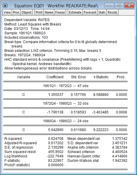
EViews reports new estimates featuring two breaks(1972Q4, 1980Q4) defining a medium, low, and a high rate regime, respectively:
The corresponding actual, fitted, residual plot is given by: