Bayesian VARs in EViews 8
One of the new features in EViews 8 is the estimation of Bayesian VARs.
VARs are frequently used in the study of macroeconomic data. Since VARs frequently require estimation of a large number of parameters, over-parameterization of VAR models is often a problem—with too few observations to estimate the parameters of the model.
One approach for solving this problem is shrinkage, where we impose restrictions on parameters to reduce the parameter set. Bayesian VAR (BVAR) methods (Litterman, 1986; Doan, Litterman, and Sims, 1984; Sims and Zha, 1998) are one popular approach for achieving shrinkage, since Bayesian priors provide a logical and consistent method of imposing parameter restrictions.
EViews supports four different prior specifications on the parameters:
- Litterman/Minnesota prior.
- Normal-Wishart prior.
- Sims-Zha Normal-Wishart prior.
- Sims-Zha Normal-flat.
Each prior type lets you additionally specify hyper-parameters for the prior, as well as initial covariance matrix assumptions.
Below we provide an example of using Bayesian VARs in EViews.
Lütkepohl 2007 Example
We estimate the coefficients of a VAR(2) model using the first differences of the logarithm of investment, income, and consumption example data. The raw data are provided in the EViews workfile wgmacro.wf1. This data set was examined by Lütkepohl (2007, New Introduction to Multiple Time Series Analysis, New York: Springer-Verlag. page 228).
View a video of this Bayesian VAR example.
Click on Quick/Estimate VAR... to open the main VAR specification dialog. In the VAR type box, select Bayesian VAR and in the Endogenous Variables box, type: dlincome dlinvestment dlconsumption.
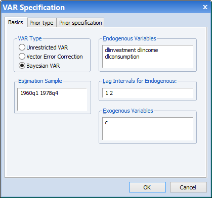
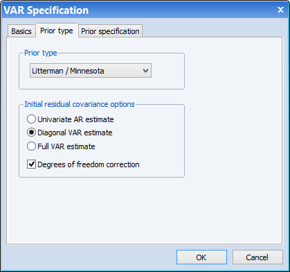
Next we switch to the Prior type tab to specify the type of prior we will use. Following Lütkepohl, we select the Litterman / Minnesota prior. By default EViews will use a univariate AR estimate for the initial covariance matrix, however we switch to using a diagonal VAR estimate (the covariance from a full standard VAR estimation, but with the off-diagonals zeroed out).
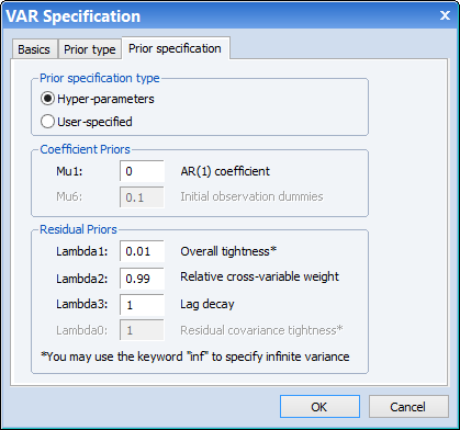
Finally, the Prior specification tab lets us specify the hyper-parameters for the prior. To match one of Lütkepohl's estimates, we set μ1 to zero, and specify a value of 0.01 for λ1, 0.99 for λ2, and 1 for λ3:
This yields the following output table:
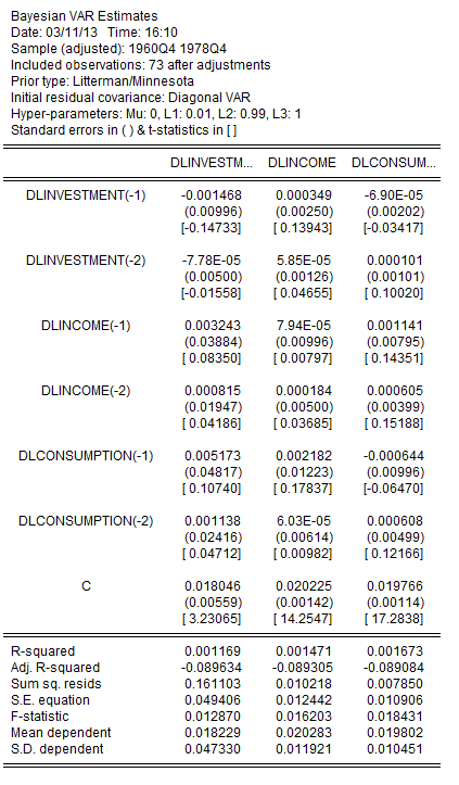
Which matches the results given in row 4 of Table 5.3 (page 228) of Lütkepohl. Note that we can match the other rows of that table by adjusting our hyper-parameter values.
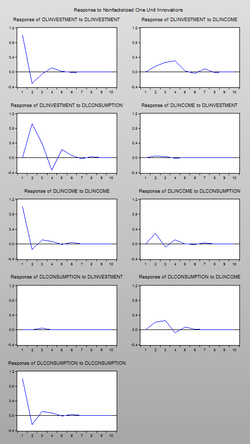
Following estimation, we can view impulse responses for the Bayesian VAR in the same way we would for any other VAR in EViews, by clicking on the Impulse button. Here we show the impulse responses for a one unit innovation, for the same BVAR estimated above, but with λ1 set to 1: