Robust Regression in EViews 8

Robust least squares, or robust regression, is one of the new features included in EViews 8.

Ordinary least squares estimators are sensitive to the presence of observations that lie outside the norm for the regression model of interest. The sensitivity of conventional regression methods to these outlier observations can result in coefficient estimates that do not accurately reflect the underlying statistical relationship.

Robust least squares refers to a variety of regression methods designed to be robust, or less sensitive, to outliers. EViews offers three different methods for robust least squares: M-estimation (Huber, 1973), S-estimation (Rousseeuw and Yohai, 1984), and MM-estimation (Yohai 1987). The three methods differ in their emphases:

M-estimation addresses dependent variable outliers where the value of the dependent variable differs markedly from the regression model norm (large residuals).
S-estimation is a computationally intensive procedure that focuses on outliers in the regressor variables (high leverages).
MM-estimation is a combination of S-estimation and M-estimation. The procedure starts by performing S-estimation, and then uses the estimates obtained from S-estimation as the starting point for M-estimation. Since MM-estimation is a combination of the other two methods, it addresses outliers in both the dependent and independent variables.

Below we provide an example of robust regression in EViews.

Outliers Example

For our example of robust regression estimation, we employ the “salinity” data set taken from Rousseeuw and Leroy (1987, Robust Regression and Outlier Detection. New York: John Wiley & Sons, Inc., page 82), which has been used in many studies of robust regression and outlier effects. See, for example, Rousseeuw and van Zomeren (1992, “A Comparison of Some Quick Algorithms for Robust Regression,”) and Fung (1993). The data consist of 28 observations on water salinity (salt concentration) and river discharge measurements taken from Pamlico Sound in North Carolina.

View a video of this detecting outliers in least squares example.

We are interested in modeling the relationship between the amount of discharge and the level of salinity. The regression model of interest is:

S_t = β₁ + β₂S_t-1 + β₃t + β₄D_t + ε_t

where S is the salinity level, D is discharge and t represents a time trend. The data are provided in the workfile Rousseeuw and Leroy.wf1. The series SALINITY and DISCHARGE contain the salt and discharge measurements, TREND contains the number of biweekly periods since the start of spring, and LAGSEL is contains the lagged value of SALINITY.

We begin with ordinary least squares estimation of this specification:

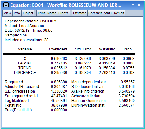
Rousseeuw and Leroy identify observation 16 as being an outlier. We can confirm this finding by looking at the influence statistics and leverages for this equation. From the EQ01 menu, display the influence statistics dialog by selecting View/Stability Diagnostics/Influence Statistics...

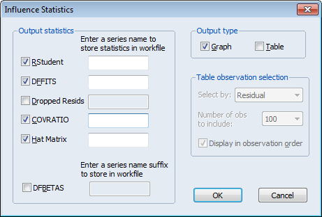
Check the box labeled Hat Matrix to tell EViews that you want to view the diagonals of the matrix along with the default results, then click on OK to display the graphs:

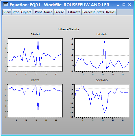
Robust Regression Influence Statistics output

The spikes in the graphs for all four influence measures point to observation 16 as being an outlier. This finding is confirmed by the leverage plot view of EQ01. Select View/Stability Diagnostics/Leverage Plots... and click on OK to accept the default settings:

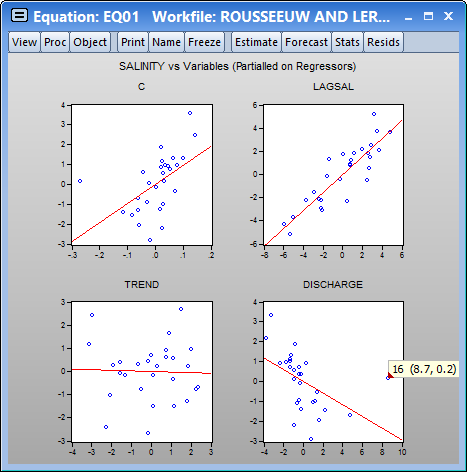
The graphs support the view that observation 16 has high leverage, especially in the relationship between SALINITY and DISCHARGE. Using the mouse pointer to hover over the outlier confirms the identity of the outlier observation.

M-Estimation

View a video of this M-Estimation example.

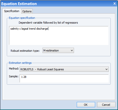
Given the presence of outliers, we re-estimate the regression using robust M-estimation. Create a new equation object by clicking on Quick/Estimate Equation…, or by selecting Object/New Object…/Equation and then select ROBUSTLS from the Method dropdown menu. Enter the dependent variable followed by the list of regressor variables in the Equation specification edit field: salinity c lagsel trend discharge and click on OK to instruct EViews to estimate the specification using the default estimator and settings.

This yields the following estimation output:

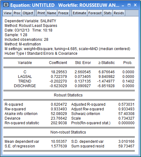
A description of the settings used in the M-estimation is presented at the top of the output. Here we see that the Bisquare function with a default tuning parameter value of 4.685 was used, that the scale was estimated using the median centered, median absolute deviation method, and that the z-statistics in the output are based on Huber Type I covariance estimates.

Turning to the coefficient estimates, we see the effect on the coefficient estimates of moving from least squares to robust M-estimation. The M-estimator produces a much larger negative impact of DISCHARGE on SALINITY than does ordinary least squares (-0.623 versus -0.295) with the M-estimator coefficient estimated with similar precision (0.091 versus 0.107). The sensitivity of the DISCHARGE coefficient estimates to robust estimation is in accord with the earlier EQ01 diagnostic suggesting that observation 16 had high leverage for the relationship between SALINITY and DISCHARGE.

The bottom portion of the output displays the R² and R²_W goodness-of-fit and adjusted measures, along which indicate that the model accounts for roughly 60-90% of the variation in the constant-only model. The statistic of 202.906 and corresponding p-value of 0.00 indicate strong rejection of the null hypothesis that all non-intercept coefficients are equal to zero. Lastly, the output shows the value of the deviance, information criteria, and the estimated scale. These measures may be of use when comparing models.

MM-Estimation

Next, we estimate the equation using MM-estimation. In the Specification tab:

Specify your equation estimation method as ROBUSTLS - Robust Least Squares,
Change the Robust Estimation Type dropdown to MM-estimation
Fill out the Specification edit field with “salinity c lagsel trend discharge” as before.

Next, we will provide values for the tuning and breakdown values, and will specify options to control the S-estimation refinement.

Click on the Options tab to display the additional estimation settings:

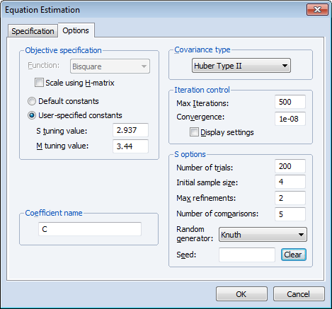
For the objective specification, we will provide tuning and breakdown values. Select the User-specified constants radio button and enter the values as depicted. The Stuning value of 2.937 is chosen to provide a breakdown of 0.25; the M-tuning value of 3.44 is chosen to produce relative efficiency of 0.85.
Select Huber Type II standard errors.
Under S options, enter values for the Number of trials, and Max refinements, as depicted. The Initial sample size will be pre-filled with the number of regressor variables specified on the first tab of the dialog—we will leave this at the default setting.
Enter “5” in the Number of comparisons edit field so that EViews will refine the best 5 of the 200 trials.

Click on OK to accept the specification and options and to estimate the equation. EViews will display the results of the MM-estimation.

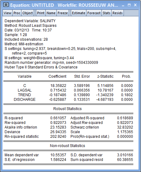
Notice that the top of the output displays various settings for both the S and the M-portions of the MM-estimation. In addition to showing the S-tuning value of 2.937 and associated breakdown value of 0.25, EViews reports that the S-estimation consists of 200 trials with initial coefficients obtained from a random initial sample size of 4 and 2 initial refinement steps. The final comparison involves fully refining 5 sets of the scale estimates and choosing the smallest scale estimate.

Once the scale estimate is obtained, EViews performs fixed scale M-estimation using the reported 3.44 tuning parameter.

EViews also reports information on the random number generator used to obtain the random subsamples, and the method used to obtain coefficient estimate covariances. Turning to the results, we note that despite the difference in robust estimation method, relative efficiency settings, and method of computing standard errors, the results from the Mestimation and the MM-estimation are generally quite similar. Most importantly, both estimates show statistically significant DISCHARGE coefficients of around -0.62 with roughly comparable coefficient standard errors (0.089 versus 0.13). The results for other coefficients are even closer.

The MM-estimate of the scale is considerably larger than that obtained from M-estimation (1.16 versus 0.73), but the overall goodness-of-fit measures and R²_N statistic and test results are quite similar.