Switching Regression and Markov Switching in EViews 8
EViews 8 new estimation features include Switching Regression (including Markov Switching).
Dynamics specifications are permitted through the use of lagged dependent variables as explanatory variables and through the presence of auto-correlated errors (Goldfeld and Quandt, 1973, 1976; Maddala, 1986; Hamilton, 1994; Frühwirth-Schnatter, 2006).
Below we provide a couple of examples of using switching regression in EViews.
Markov Switching AR
Hamilton (1989) specifies a two-state Markov switching model in which the mean growth rate of GNP is subject to regime switching, and where the errors follow a regime-invariant AR(4) process. The data for this example, which consists of the series G containing (100 Examples—409 times) the log difference of quarterly U.S. GNP for 1951q1–1984q4, may be found in the workfile GNP_hamilton.WF1.
View a video tutorial of Markov Switching.
To estimate the Hamilton model, open a switching equation dialog and enter the specification as depicted below:
The equation specification consists of a two-state Markov switching model with a single switching mean regressor C and the four non-switching AR terms. The error variance is assumed to be common across the regimes. The only probability regressor is the constant C since we have time-invariant regime transition probabilities.
With the exception of the convergence tolerance which we set to 1e-8, we leave the rest of the settings at their default values. Click on OK to estimate the equation and display the estimation results.
The top portion of the output describes the estimation settings:
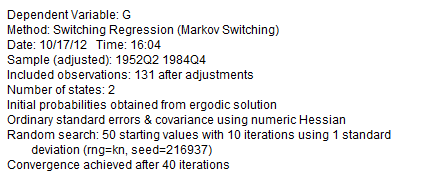
(Bear in mind that if you attempt replicate this estimation using the default settings, you may obtain different results due to the different set of random starting values. You may use the random number generator seed settings to obtain the same starting values.) The middle section displays the coefficients for the regime specific mean and the invariant error distribution coefficients. We see, in the differences in the regime specific means, what Hamilton terms the fast and slow growth rates for the U.S. economy.
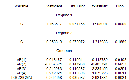
The remaining results show the parameters of the transition matrix and summary statistics for the estimated equation.
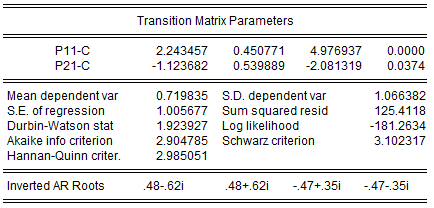
Instead of focusing on the transition matrix parameters, we examine the transition matrix probabilities directly by selecting View/Regime Results/Transition Results... and clicking on OK to display the default summary view:
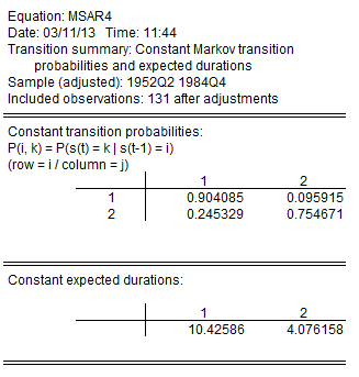
Here, we see the transition probability matrix and the expected durations. Note that there is considerable state dependence in the transition probabilities with a relatively higher probability of remaining in the origin regime (0.90 for the high output state, 0.75 for the low output state). The corresponding expected durations in a regime are approximately 10.4 and 4.1 quarters, respectively.
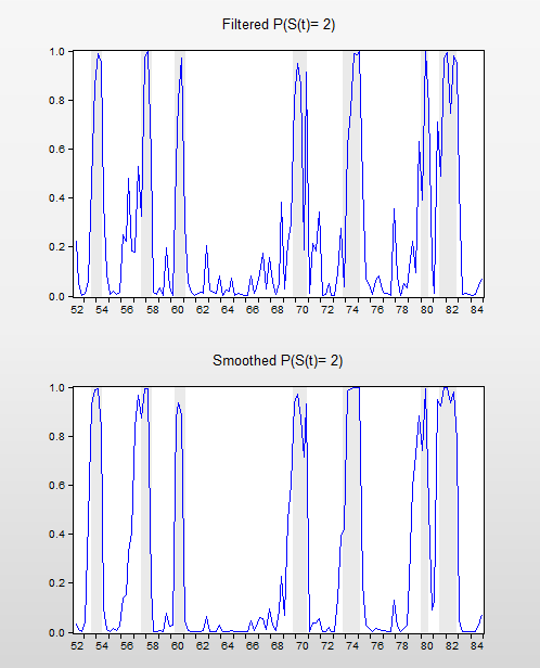
Lastly, we display the filtered and full sample estimates of the probabilities of being in the two regimes. First select View/Regime Results/Regime Probabilities... and choose the filtered results. We will display the results only for the second regime. Then repeat the procedure choosing the smoothed results.
After saving the two views as graphs, editing the labels, and applying the RecShade add-in (http://www.eviews.com/Addins/addins.shtml) to label the NBER recessions, we see that the predicted probabilities of being in the low output state coincide nicely with the commonly employed definition of recessions:
Time-Varying Transitions
Kim and Nelson (1999, p. 93) provide example data for estimating an MSAR(4) model with time-varying transition probabilities, as in Filardo (1994). Filardo models the log growth rate of industrial production (DLOGIP) using an MSAR(4) switching mean specification, using (among other variables) the log growth rate of the Composite Index of Eleven Leading Indicators (DLOGIDX) as a business-cycle predictor.
The Kim and Nelson monthly data for 1948m01 to 1991m04 are included the workfile kimnelson_tvp.WF1. Note that these data correspond to, but differ slightly from the data used in Filardo (1994).
We open the switching regression dialog and fill out the Specification tab with the switching mean AR(4) spec and the switching probability specification:
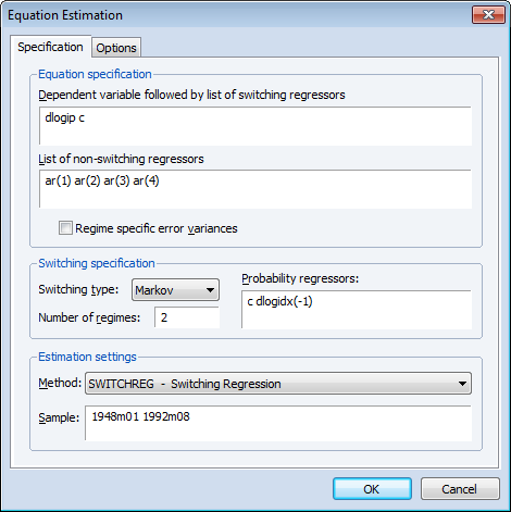
Note that use have used the lag of the leading indicator variable as our probability regressor so that the t period data for the regressor corresponds to the values influencing the transitions for t-1 to t.
We leave the remaining settings at their defaults and click on OK to estimate the equation. Following estimation, EViews displays the results:
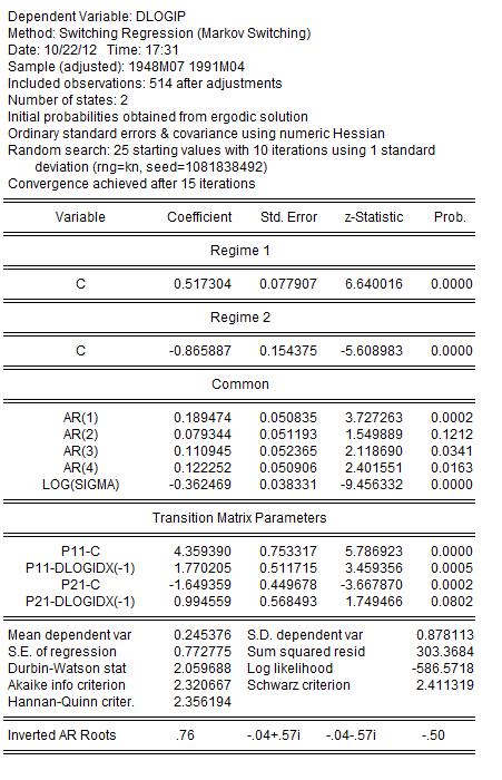
The results are broadly similar to, but differ slightly from those reported by Filardo. The coefficients on the DLOGIDX(-1) both differ from zero with opposite (statistically significant) signs. As to the transition matrix parameters, we see that increases in the log growth rate are associated with higher probabilities of being in the high production growth regime, lowering the transition probability out of regime 1 and increasing the transition probability from regime 2 into regime 1.
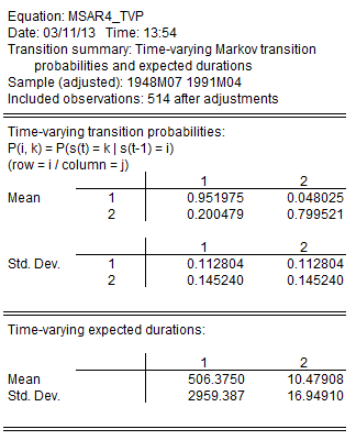
We can examine more directly the transition probabilities. The default transition probability summary (View/Regime Results/Transition Results...) shows descriptive statistics for the elements of the transition matrix:
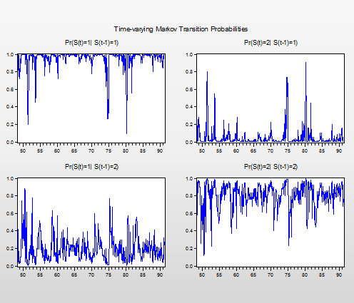
We can see the variation in the time-varying probabilities by examining graphs of the transition probabilities for each observation. Select View/Regime Results/Transition Results... and click on the Transition probabilities radio button. The default view for showing the probabilities is a graph so you may simply click on OK to show graphs for all four probabilities.
The filtered probabilities of being in the low production regime are presented below, with NBER recession shading.
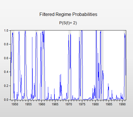
To create this graph, select View/Regime Results/Regime Probabilities..., select the Filtered radio button and enter “2” in the Regimes to plot edit field to only show the second (low production) regime.
Click on OK to display the graph view, then click on the Freeze button to save the view as a graph object. Select Proc/Add-ins/Add USA Recession Shading in the graph menu (you must first install the RecShade Add-in to use the automatic shading feature — http://www.eviews.com/Addins/addins.shtml).
Regime Heteroskedasticity
Kim and Nelson (1999) offer an example (Section 4.6, p. 86) of a three state Markov switching model of regime heteroskedastic stock returns from 1926m1–1986m12. The data, which consist of monthly CRSP equal-weighted excess returns are in the series EXCESS, provided in the workfile ew_excs.WF1.
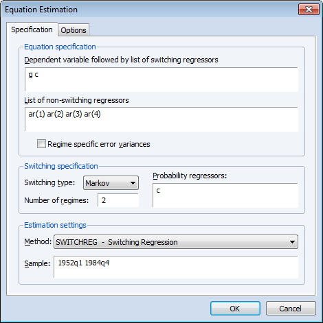
The specification of the model is as depicted in the dialog below:
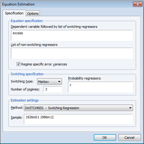
The excess returns are assumed to have mean zero so we enter only the name of the dependent variable in the topmost edit field. Since we wish to model regime heteroskedasticity, Regime specific error variances box is checked. The model assumes Markov switching probabilities with 3 regimes and constant transition probabilities.
Preliminary analysis indicates that this model is particularly difficult to estimate with a number of local roots exhibiting coefficient singularity.
To obtain estimates we instruct EViews to perform extra randomized starting value estimation. Click on the Options tab and change the starting value settings so EViews generates 50 sets of random starts (instead of 25) with 20 (instead of 10) iteration refinements. Click on OK to proceed with the estimation.
EViews estimates the model and displays the standard switching regression output:
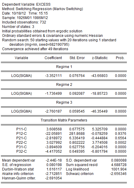
The results show estimates of the log standard deviations in the low, high, and medium volatility regimes. The implied standard deviations are 0.035, 0.176, and 0.063, respectively.
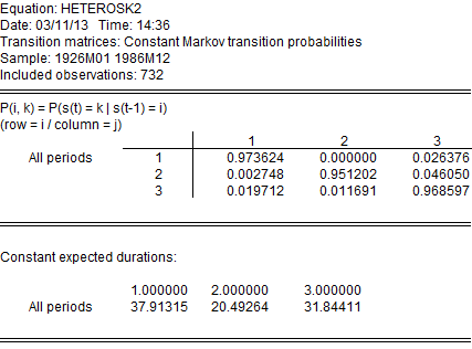
We may view the estimated transition probability matrix by clicking on View/Regime Results/Transition Results... and clicking on OK to display the summary:
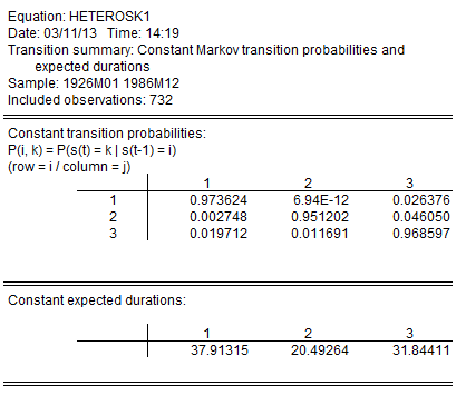
The transition probabilities point to a possible explanation of the difficulty in estimating the model. The transition probability from the low volatility regime 1 to the high volatility regime 2 is essentially zero.
We may impose a zero restriction on transitions from the high to low state by creating a 3 X 3 matrix object RESTR containing:
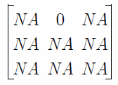
and re-estimating the model using this restriction matrix. One tricky aspect of imposing restrictions is that the regime identities are not fixed and can change for different starting values. Accordingly, we re-estimate the model using the prior coefficient estimates as user-specified starting values, keeping in mind that the P12-C coefficient no longer exists.
Your example workfile includes the vector object STARTCOEFS which contains the coefficient estimates from the unrestricted equation with the P12-C coefficient removed. Select Proc/Set Global Coefs from the STARTCOEFS toolbar to place these values in the C coefficient vector.
Next, go to the original equation and make a copy by selecting Object/Copy Object. Click on the Estimate button go to the Options tab, enter the name of the restriction vector in the Transition prob restr. matrix edit field, and change the Start method to User Specified.
Click on OK to accept the changes and estimate the equation. The update results are displayed below:
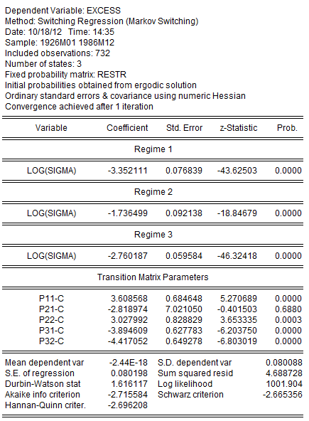
Note that the coefficient associated with the restricted probability p12 has been removed. The transition probabilities view shows us the updated probabilities with the restricted value for p12: